5 Point-Slope Form Examples with Simple Explanations

5 Point-Slope Form Examples for Students

When it comes to graphing lines on the coordinate plane, there are several different ways to express a linear equation and figure out how to determine a given line’s slope, y-intercept, points it passes through, and what its graph looks like. Being able to understand and solve problems involving linear equations in various forms, including point-slope form, is an immensely useful and important algebra skills that will help you to solve math problems involving linear equations.

The following lesson will take you step-by-step through solving 5 point-slope formula examples (sample problems) that we will solve and find the final correct answer together. By working through these 5 examples, you will gain a much better understanding of point-slope formula, what it means, and how to use it to solve problems on future homework assignments, quizzes, tests, and exams.

But, before we start working on the point-slope form examples, we will quickly review some very important vocabulary terms and review some key information regarding lines, equations, slopes, and y-intercepts. It is helpful to review this information, even if you are already familiar with it, as you will be building upon it as this lesson progresses and having a strong foundation makes a world of difference.

What is Point-Slope Form?

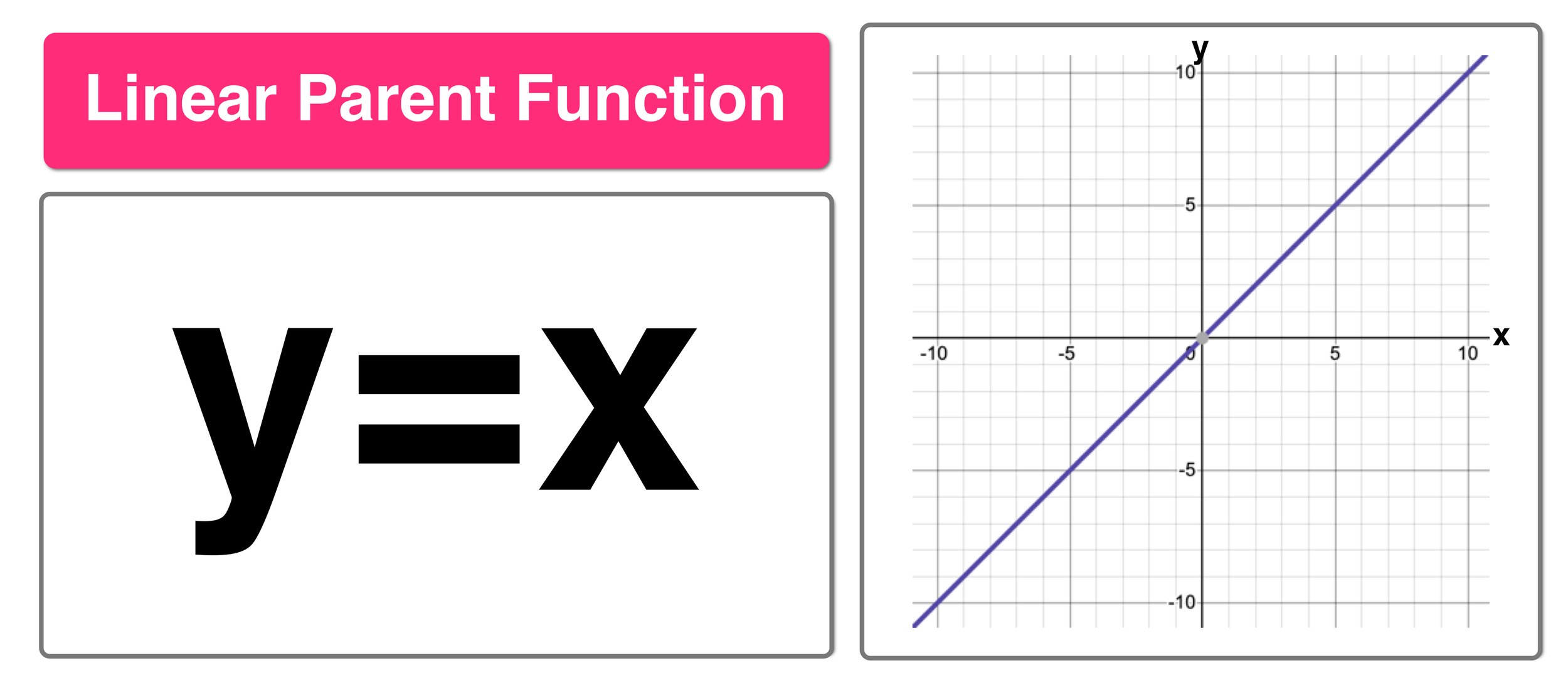
In math, there are more than one way to express the equation of a line (also referred to as a linear equation).

Most algebra students first learn about slope-intercept form: y=mx+b, where m equals the slope of the line and b equals the y-intercept.

With slope-intercept form, as long as you know the slope and y-intercept of the line, you can determine its equation, graph the line on the coordinate plane, and figure out what points the line passes through.

What is point-slope form?

Definition: The point-slope form of a line is expressed using the slope of the line and point that the line passes through.

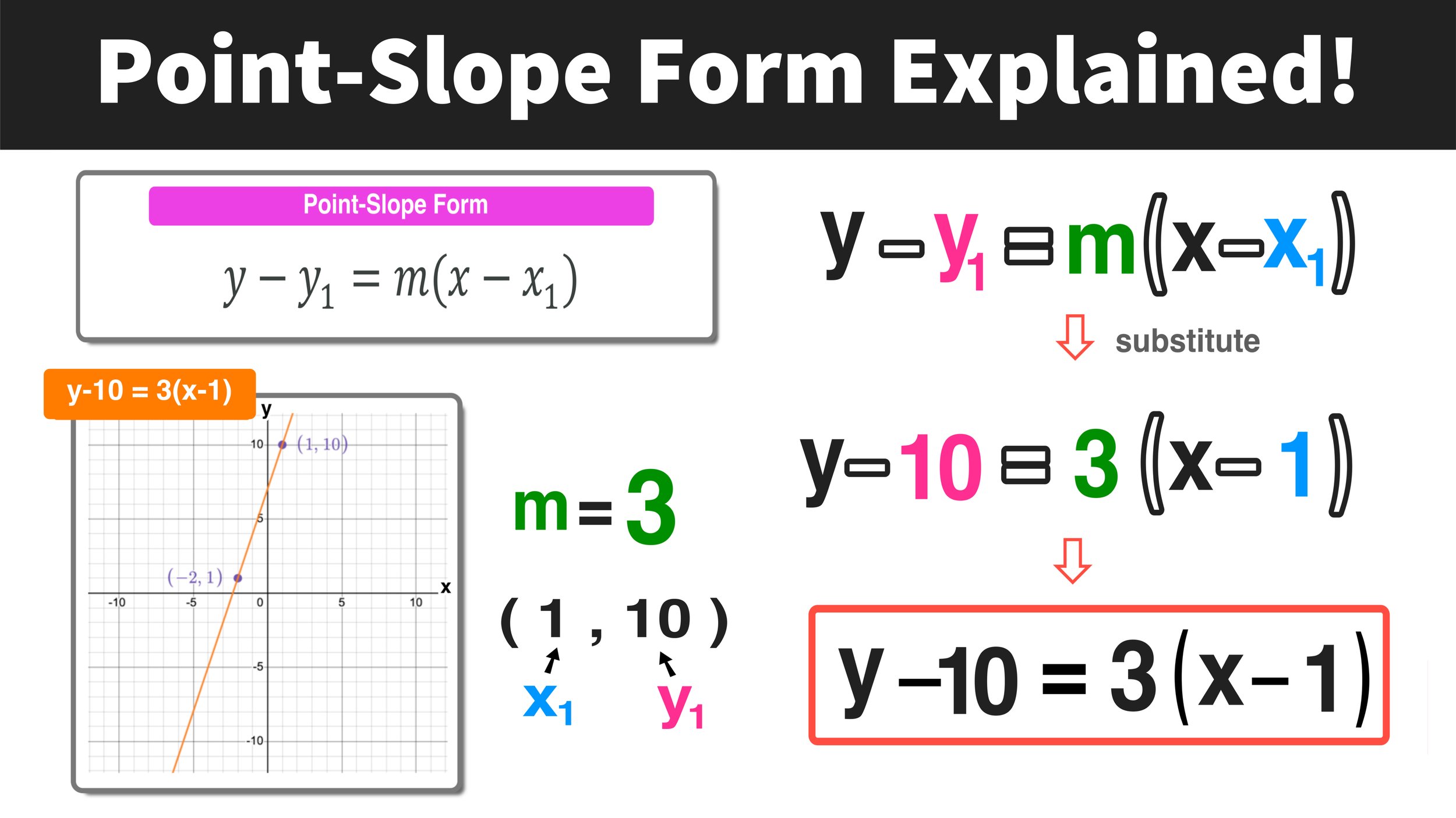
Formula: y-y1 = m(x - x1) where m equals the slope of the line and x1 and y1 equal the corresponding x- and y-coordinates of a given point the line passes through.

Unlike slope-intercept form, point-slope form does not require you to know the function’s y-intercept. Instead, you are only concerned with the slope and the coordinates of one point that the line passes through.

If you find this definition confusing, take a look at the graphic below that compares slope-intercept form and point-slope form and further analyze the key similarities and differences between the two forms.

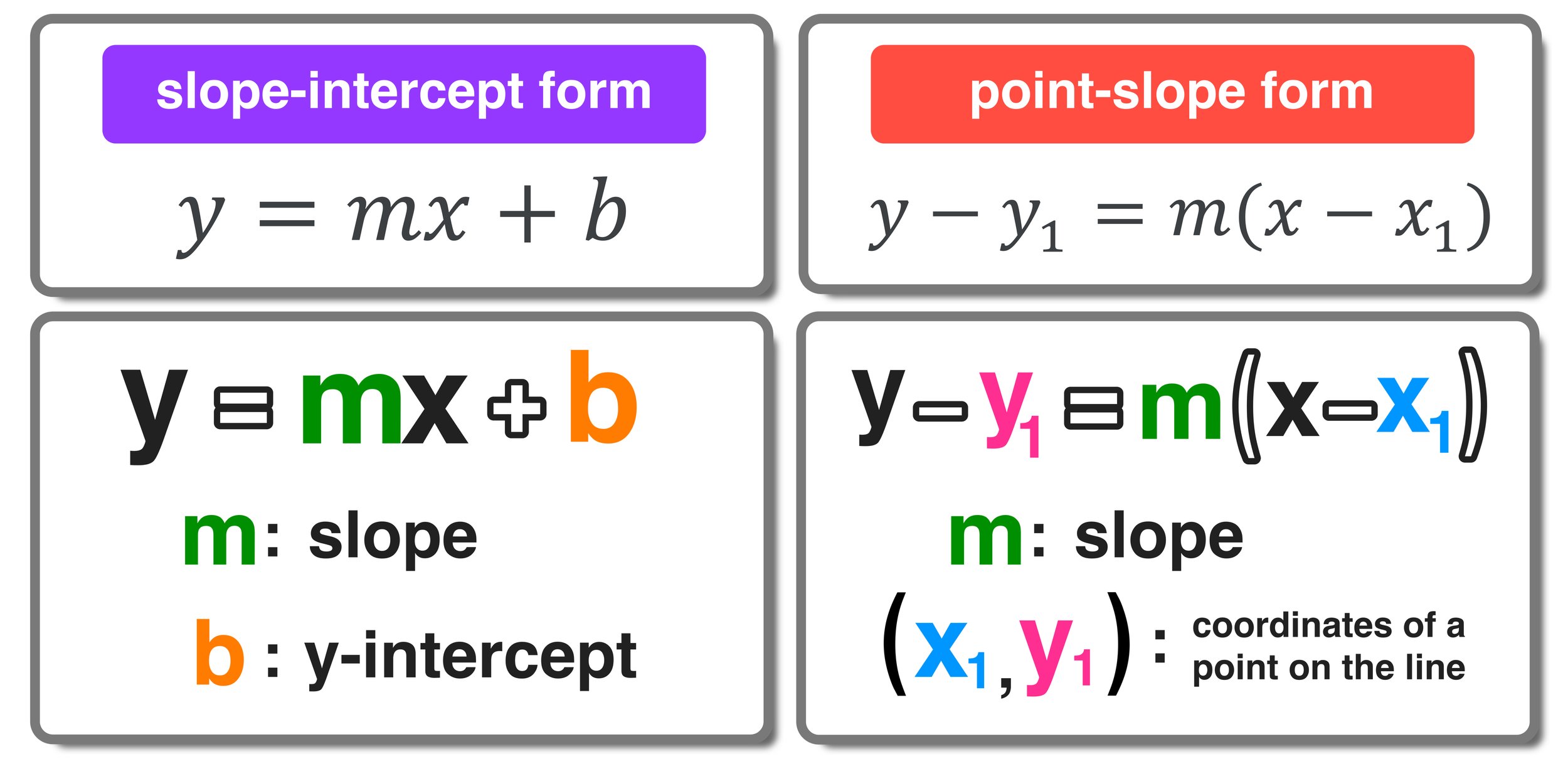
In terms of similarities, both slope-intercept and point-slope form require you to know the slope of the line.

(Looking to learn how to find the slope of a line? click here to access our free guide )

However, the key difference is that slope-intercept form requires you to know the y-intercept of the graph, while point-slope form requires you only to know the coordinates of one point that the graph passes through (this point can be anywhere on the line).

Now that you are familiar with the point-slope form formula, you are almost ready to work through some point-slope form examples. But, before we explore point-slope form further, let’s take a quick look two simple situations involving graphing linear functions using given information.

▶ Situation A: Graph the Linear Function

Problem: Graph a line with a slope of 3 and a y-intercept at 6 and write its equation in y= form.
Notice that Situation A gives us enough information right from the start to write the equation in y=mx+b form since we already know the slope, m, and y-intercept b.

• m=3 and b=6

 We can write the equation as follows:

•  y=3x+6

 This line has a slope of 3 (or 3/1) and a y-intercept at positive 6. We can now graph this line as follows:

Situation B▶: Graph the Linear Function

 Problem: Graph a line with a slope of 3 that passes through the point (2,12) and write its equation in y= form

Notice that situation B does not give us enough information to write the equation of the line in y= form since we only know the slope and not the y-intercept.

 This is where point-slope form comes into play!

In cases like this, m represents the slope, which is 3 and x1 and y1 are the corresponding x- and y-coordinates of whatever given point the line passes through.

Since we already know that the line passes through the point (2,12), we know that x1=2 and y1=12 

We can substitute these values into the point slope formula as follows

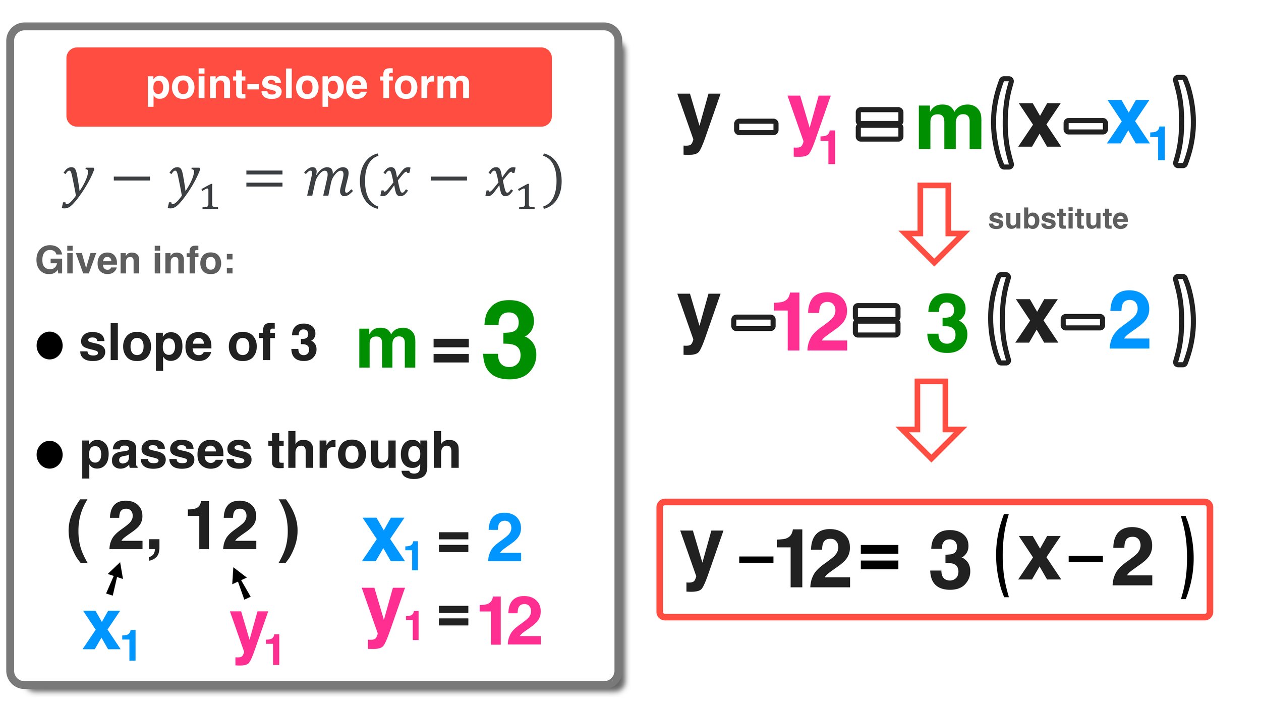
 After substituting m=3, x1=2, and y1=12, you end up with the following equation in point-slope form:

• y-12 = 3(x-2) 

If we want to graph the line on the coordinate plane, it may be easier to rearrange this formula into y=mx+b form as follows:

To convert from point-slope form to slope-intercept form:

• y-12=3(x-2) ➞ y-12=3x-6 ➞ y=3x+6

Now that we have converted the equation into y=mx+b form, we can go ahead and graph this line since we know that the slope is 3 and the y-intercept is positive 6.

Notice that the line does pass through the point (2,12).

What else do you notice about this graph? It turns out that situation A and situation B both represent the same linear equation, just in different forms.

• Situation A: slope-intercept form

• Situation B: point-slope form

If you are comfortable with solving problems involving equations in y=mx+b form (slope-intercept form), then you can surely be successful at solving problems involving point-slope form (y-y1=m(x-x1).

To take this next step, practice is key! So, now let’s look at 5 examples of solving algebra problems involving point-slope form to give you some more experience.

---

---

Point-Slope Form Example #1

Problem: Determine the point-slope form of a line that has a slope of 1/2 and passes through the point (8,2).

To determine the equation of this line in point-slope form, you have to know the following pieces of information:

• the slope of the line, m

• the coordinates of a point that the line passes through, (x1, y1)

In this first example, both of these pieces of information are given to you, so you are ready to write the equation of the line in point-slope form by substituting m=1/2, x1=8, and y1=2 as follows:

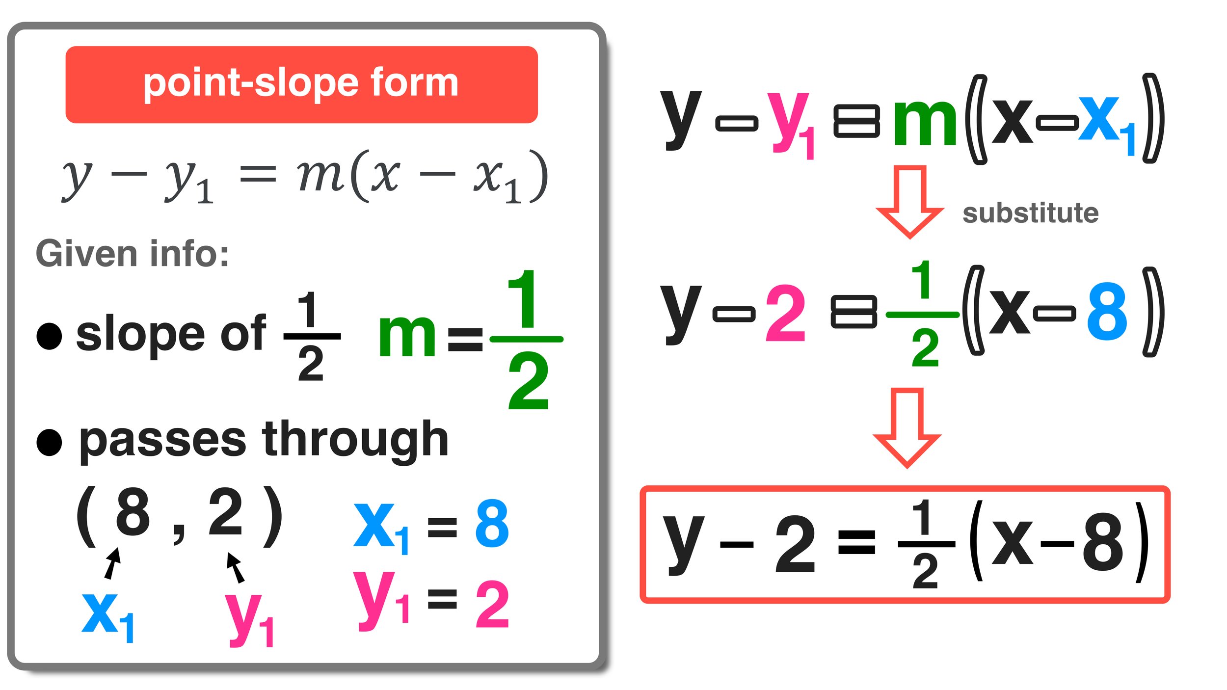
Answer: The equation of the line in point-slope form is: y-2=1/2x(x-8)

---

Point-Slope Form Example #2

Problem: Determine the point-slope form of a line that has a slope of 3/4 and passes through the point (4,-6).

Again, to determine the equation of this line in point-slope form, you have to know the following pieces of information:

• the slope of the line, m

• the coordinates of a point that the line passes through, (x1, y1)

Just like example #1, both of these pieces of information are given to you, so you are ready to write the equation of the line in point-slope form by substituting m=3/4, x1=4, and y1=-6 as follows:

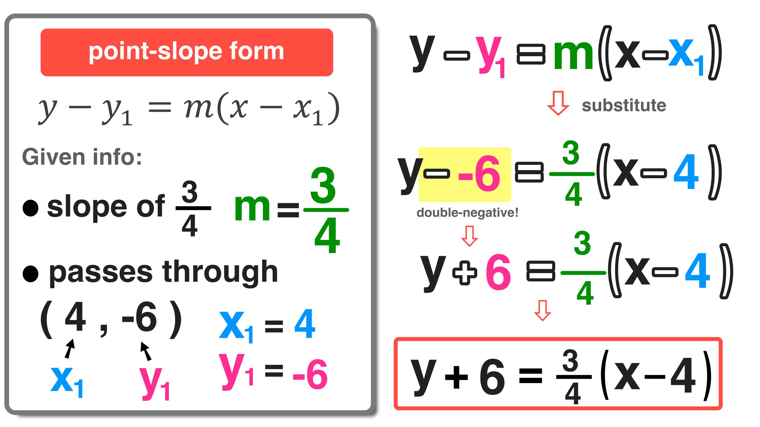
In this example, the value of y1 is a negative number (-6). When you substitute this value into the point-slope formula, on the left-side of the equation, you end up with: y - - 6

You can simplify this double-negative by rewriting it as a positive: y- -6 ➞ y + 6

Answer: The equation of the line in point-slope form is: y+6=3/4x(x-4)

---

Point-Slope Form Example #3

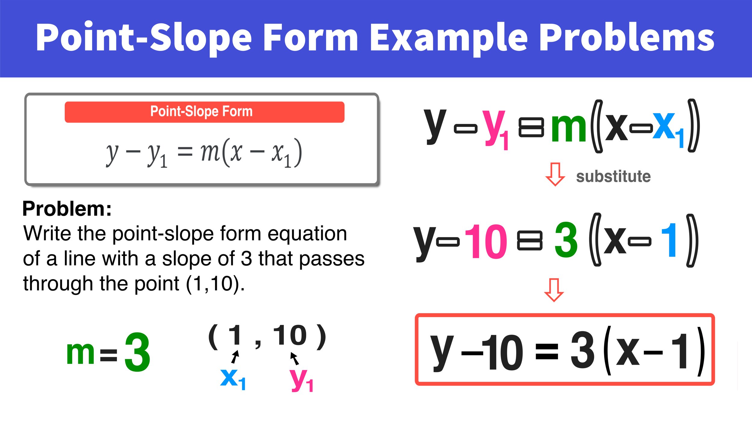
Problem: Determine the point-slope form of a line that passes through the points (1,10) and (3,16)

Just like the previous two examples, to determine the equation of this line in point-slope form, you have to know the following pieces of information:

• the slope of the line, m

• the coordinates of a point that the line passes through, (x1, y1)

Unlike the first two examples, in this case you are not given all of the required information upfront. While you know that coordinates of a point that the line passes through (you actually know two of them), you do not know the slope of the line.

Luckily, you can use the slope formula to find the slope of a line that passes through two given points.

The slope formula is equal to change in y over change in x.

To correctly use the slope formula, you have to correctly label and identify the (x1, y1) and (x2, y2) values so you can substitute them into the formula. The first point that you use will have the 1’s and the second point that you identify will have the 2’s.

• (1) First Point: (x1,y1) ➞ (1,10) where x1=1 and y1=10

• (2) Second Point: (x2,y2)➞ (3,16) where x2=3 and y2=16

You are now ready to calculate the slope as follows:

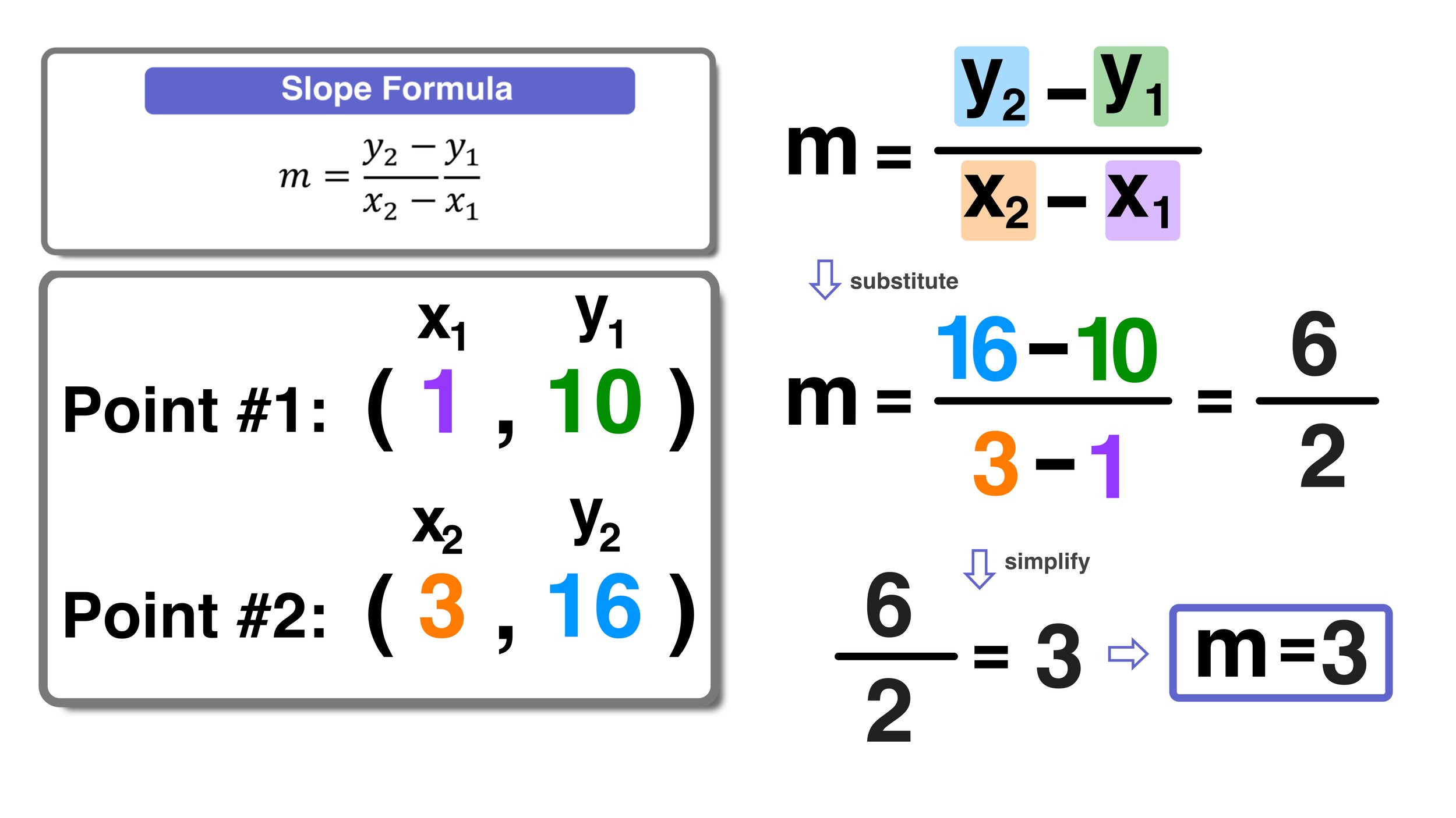
By substituting the values of (x1,y1) and (x2,y2) into the slope formula, you end up with :

• m = (16-10)/(3-1) = 6/2 = 3

After simplifying 6/2 to 3, you can conclude that the slope of the line, m, equals 3

Now that you know the slope of the line and the coordinates of a point that the line passes through, you can write the equation of the line in point-slope form. Note that you can choose either given point that the line passes through (1,10) or (3,16). Below, we will use the first given point (1,10):

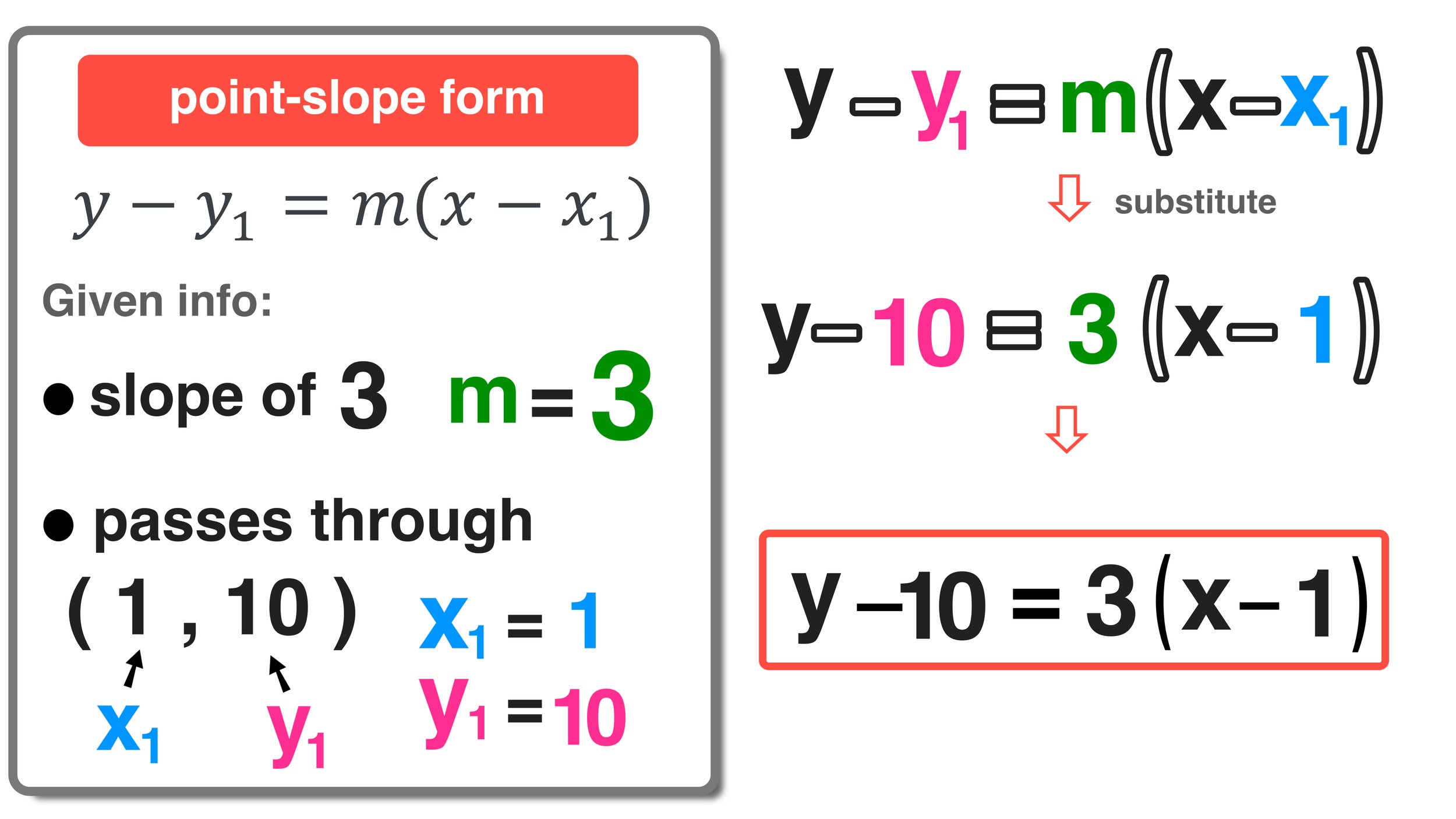
Answer: The equation of the line in point-slope form is: y-10=3(x-1)

---

Point-Slope Form Example #4

Problem: Determine the point-slope form of a line that passes through the points (-5,15) and (-10,18)

Again, in order to determine the equation of this line in point-slope form, you have to know the following pieces of information:

• the slope of the line, m

• the coordinates of a point that the line passes through, (x1, y1)

Just like in example #3, you are not given all of the required information upfront. While you know that coordinates of a point that the line passes through, you do not know the slope of the line.

Following the same process as example #3, you can use the slope formula to determine the value of m as follows:

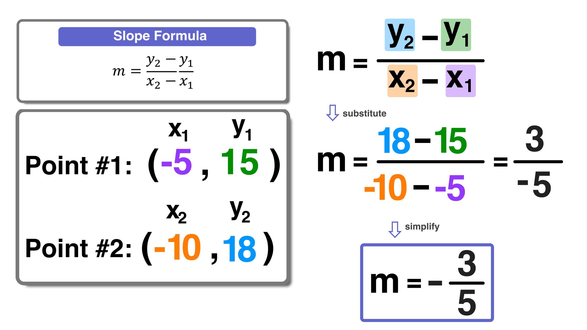
By substituting the values of (x1,y1) and (x2,y2) into the slope formula, you end up with :

• m = (18-15)/(-10- -5)

Notice that the double negative in the denominator can be rewritten as: (-10- -5) ➞ (-10 + 5)

• m = (18-15)/(-10 + 5) = 3/-5

You can express these results as -3/5, so you can conclude that the slope of the line, m, equals -3/5

Now that you know the slope of the line and the coordinates of a point that the line passes through, you can write the equation of the line in point-slope form. Just like the last example, you can choose either given point that the line passes through (-5,15) or (-10,18). Below, we will use the first given point (-5,15):

Answer: The equation of the line in point-slope form is: y-15=-3/5(x+1)

---

Point-Slope Form Example #5

Problem: Graph the line with the following point-slope form equation: y-4=2(x+6)

In this final example, you will have to graph a line and all that you are given is a linear equation in point-slope form.

All that you need to graph a line is the slope of the line and a point that the passes through—which is exactly what you can find when you look at the equation in point slope form.

Remember that point slope form is as follows: y-y1 = m(x = x1) where m equals the slope of the line and (x1,y1) are the corresponding x- and y-coordinates of the point the line passes through.

So, in this example, we can see that the slope of the line m=2 (or 2/1)

Furthermore, we can see that the y1=4, but what about x1?

Since we see that ‘+’ sign on the right-side of the equation (x+6), we know that a double-negative must have occurred, so the x1 value is equal to -6 (not positive 6).

Now we have all of the information that we need:

• Slope: m=4

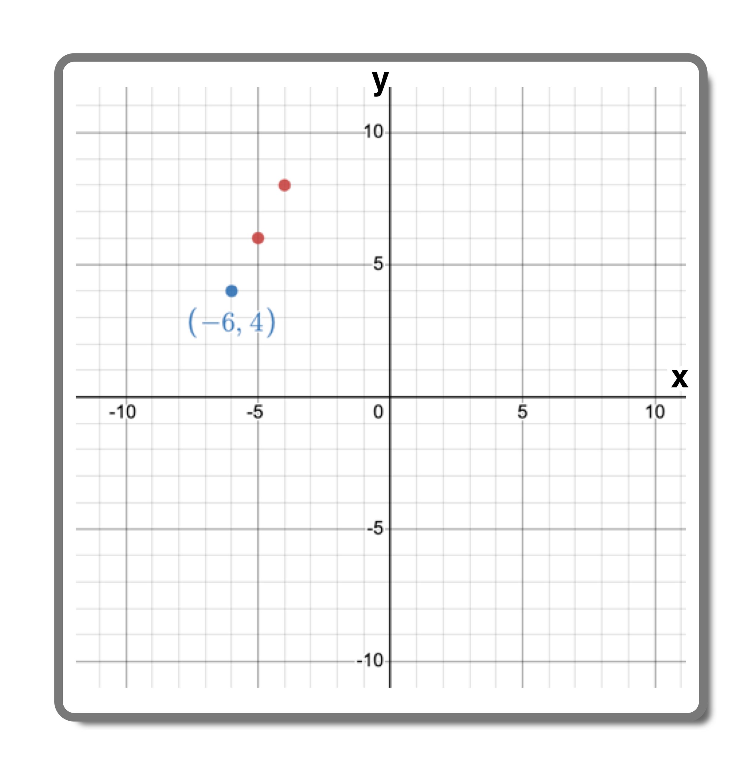
• Point: (x1,y1) = (-6,4)

All that we have to do now is graph the line. Start by plotting the (x1,y1) point, which is (-6,4) in this example as follows:

Next, use the slope m=2/1 to “build” more points by using the rise over run method (rise two units, and run two units to the right) as follows:

Finally, draw the line that intersects the points that you plotted to complete your graph:

Answer:

---

Keep Learning:

Calculating Percent Decrease in 3 Easy Steps

Calculating Percent Decrease in 3 Easy Steps

Being able to calculate percent decrease is an extremely useful and important numerical skill that can has implications far beyond the math classroom. An ability to calculate, understand, and analyze percents will not only help to excel on quizzes, tests, and examples, but in real world situations as well. While students often believe that calculating percent decrease to be challenging task, the process to getting correct answers is actually very easy and straightforward.

(Looking for a Percent Decrease Calculator to make a super-fast calculation: Click here to access our free Percent Decrease Calculator)

The following free Calculating Percent Decrease step-by-step lesson guide will walk you through calculating percent decrease using an easy and simple three-step method. By learning to follow these three steps, you will be able to quickly and accurately solve problems in math involving percent decrease.

Before we start learning about calculating percent decrease and the three-step method, lets perform a fast review of a few important math vocabulary terms and concepts related to this topic.

Looking to learn how to calculate percent increase or percent change? Use the links below to download our free step-by-step guides:

• How to calculate the percent increase between two numbers

• How to calculate the percent change between two numbers

Percent Definition

In mathematics, the term percent refers to parts per one hundred and the mathematical symbol for percent is %.

For example, the value 40% is defined as 40 per 100. If you observe the below diagram, you will see that the blue shaded region makes up 40% of the entire grid.

We can also say that percent represents a ratio of a value out of one hundred.

Another example would be 20% meaning 20 out of every 100. Looking at percent as a ratio, when can say that if 20% of 300 students have an exam on Monday, then 60 total students have an exam on Monday (20 out of every hundred means three 20’s out of 300 total students).

Percent Decrease Definition

The next question we have to ask is what is the meaning of percent decrease?

In mathematics, the percent decrease between two values is the difference between the final number and the initial number (which we will refer to as the starting number in this guide). Percent decrease is always expressed as a percentage of the starting number.

Note that percent decrease is a value that will be expressed as a percentage and will include the % symbol.

For example, if you had $80 dollars in savings at the start of the month and $60 in savings by the end of the month and you needed to calculate the percent decrease, the final number would be 60 and the starting number would be 80.

Being able to correctly identify the starting number and the final number is extremely important when it comes to correctly solving percent decrease problems.

Calculating Percent Decrease

Now it’s time for you to learn how to calculate percent decrease using our simple three-step method.

Let’s revisit the previous scenario involving money in your savings account decreasing between the start of the month and the end of the month:

Calculating Percent Decrease Example #1

For the first example, let’s find the percent decrease for the following scenario:

If a total amount in your savings account of $80 at the start of the month had decreased down to $60 by the end of the month, what is the percent decrease?

Here is how you can apply our three-step method:

Step 1: Find the difference of the values by subtracting the final value from the starting value.

In this example, the difference of starting value and the final value can be calculated as follows:

80 – 60 = 20

In this case, the difference of the two values would be 20. Note that, when calculating percent decrease, you will always be subtracting the smaller value from the larger value.

Step 2: Divide the difference by the starting number.

The next step is to take the difference (20 in this example) and divide it by the starting number (80 in this example) as follows:

20/80 = 0.25

Always express your answer as a decimal (this is crucial for performing your final calculation in Step 3).

Step 3: Multiply by 100

The third and final step is to multiply the decimal result from Step 2 by 100 and then express that result as a percent using the % symbol.

0.25 x 100 = 25

Final Answer: 25% Decrease

You’re done! By using the three-step method, you can conclude that there was a 25% decrease in how much money you had in savings from the start of the month to the end of the month.

Need more help? No worries. Let’s move onto another example where we will calculate percent decrease using the same three-step method.

---

Looking for a free Percent Decrease Calculator?

If you need a faster way to calculate the percent decrease between two numbers, check out our free Percent Decrease Calculator tool, which lets you input the starting and final values to get an instant answer!

▶ Click here to access our free Percent Decrease Calculator for students

---

Calculating Percent Increase Example #2

Last week, Zoe sold a total of 51 chocolate cupcakes at her bakery. This week, she sold a total of 34 chocolate cupcakes at her bakery. What was the percent decrease in the total amount of chocolate cupcakes sold between last week and this week?

To solve this problem, note that the starting value is 51 and the final value is 34.

Step 1: Find the difference of the values by subtracting the final value from the starting value.

In this example, the final value minus the starting value can be calculated as follows:

51– 34 = 17

Step 2: Divide the difference by the starting number.

For step two, take the difference (17 in this example) and divide it by the starting number (51 in this example) as follows:

17/51 = 0.3333333…

Notice that the result is a repeating/non-terminating decimal. You can round this result to the nearest hundredths decimal place to make things easier. In this case, you can round the result to 0.33

Step 3: Multiply by 100

The last step is to multiply the decimal result from step two by one hundred and express the final result as a percent. So…

0.33 x 100 = 33

 Final Answer: 33% Decrease

We’re all finished! We have concluded that there was a 33% decrease in the total amount of chocolate cupcakes sold at Zoe’s Bakery between last week and this week.

After this first example, you should be feeling more confident about your ability to correctly calculate percent decrease e using the three-step method. Let’s gain some more experience by looking at another example.

---

Calculating Percent Decrease Example #3

Last school year, 414 students attended the Delta High School Winter Ball This year, only 112 students attended the Delta High School Winter Ball. What was the percent decrease in students who attended the Winter Ball between last year and this year?

 Just like the last two examples, you can solve this problem by following the three-step process:

Step 1: Find the difference of the values by subtracting the starting value from the final value.

 In this example, the starting value minus the final value can be calculated as follows:

414– 112 = 302

Step 2: Divide the difference by the starting number.

Let’s continue with step two as follows:

Find the difference (190 in this example) and divide it by the starting number (414 in this example) as follows:

302/414 = 0.7294685…

Just like in example 2, you can round the result to the nearest hundredths decimal place to make things easier. In this case, you can round the result to 0.73

Step 3: Multiply by 100

The last step is to multiply the decimal result from step two by 100 and express the final result as a percent. So…

0.73  x 100 = 73

Final Answer: 73% Decrease

At this point, you should feel much better about your ability to calculate percent decrease and solve any math problems involving percent decrease our three-step method. But, if you feel like you need more practice, it is highly recommended that you work through examples one through again on your—be sure to do the problems by hand and take notes as you go along!

Conclusion: Calculating Percent Decrease

You can calculate percent decrease given any two values by using the following 3-step method:

Step 1: Find the difference of the values by subtracting the final value from the starting value.

Step 2: Divide the difference by the starting number. Express result as a decimal.

Step 3: Step 3: Multiply by 100. Express result as a %.

---

What about Calculating Percent Increase and Percent Change?

Learn how to calculate a percent increase or a percent change between two numbers using our free step-by-step guides. Click the links below to get started.

⇥ Calculating Percent Increase in 3 Easy Steps

⇥ Calculating Percent Change in 3 Easy Steps

---

Don’t forget about our Free Percent Decrease Calculator

Click here to get started using our free Percent Decrease Calculator

---

Keep Learning:

Where is the hundredths place value in math?

Where is the hundredths decimal place in math?

In math, when we look at numbers, we can assign something called place value to each digit based on the position of each number.

When learning about and analyzing numbers—ranging from simple single-digit numbers all the way up to extremely large numbers that can have ten digits or more or—it is important that you understand the meaning of the significance of each digit’s place value, especially when decimals are involved.

When you first start learning about place value, determining each digit’s place value can be simple, especially when you are dealing with integers and decimals are not involved. However, once decimals are in play, identifying place value can get a bit trickier.

This free and simple guide for students will focus on the hundredths place and can be used as a quick review to help you along your place value journey when you start working with numbers involving decimals.

Once you understand place value, you will gain a deeper understanding of numbers—large and small—and your mental math and operational skills (performing addition, subtraction, multiplication, division, and more) will surely improve.

Are you ready to get started?

What is place value?

Before we learn about the hundredths place and what it means in terms of place value, let’s do a super quick review of some key vocabulary terms and some things that you may already know.

Definition: In math, place value refers to the numerical value that a digit has by virtue of its position in the number.

For example, consider the number 2.5.

We can think of the number 2.5 as the sum of 2 ones and 5 tenths.

So, in terms of place value, we can say that for the number 2.5:

•  2 is in the ones place

• 5 is in the tenths place

Pretty simple, right? Now, let’s extend this understanding of place value to the hundredths place.

 What is the hundredths place?

In our last example, we looked at 2.5, which is a relatively simple decimal. As numbers grow larger, you will have to identify larger types of place values.

For example, consider the number 2.54.

We can express the number 2.54 as the sum of 2 ones, 5 tenths, and 4 hundredths.

So, in terms of place value, we can say that for the number 2.54:

•  2 is in the ones place

• 5 is in the tenths place

• 4 is in the hundredths place

In these previous examples, we are essentially deconstructing each number to identify the place value of each digit.

Note that the tenths place is different than the tens place and the hundredths place is different than the hundreds place.

 The chart below shows you each place value position relative to a decimal point.

For example, consider the number 539.25

We can insert this value into the chart as follows:

Using the chart, we can clearly see that

• 5 is in the hundreds place

• 3 is in the tens place

• 9 is in the ones place

• 2 is in the tenths place

• 5 is in the hundredths place

 Be sure not to confuse the hundreds place with the hundredths place!

Hundredths Decimal Place Examples

Now let’s go ahead and look at some more examples of determining which number is in the hundredths decimal place of a given number.

Example #1: Which digit is in the hundredths decimal place?

216.325

 We can input this value into our chart as follows.

Using the chart, it is easy to see that the value in the hundredths place is 2.

 216.325

 Answer: 2

Example #2: Which digit is in the hundredths decimal place?

0.791

We can input this value into our chart as follows.

Using the chart, it is easy to see that the value in the hundredths place is 9.

0.791

Answer: 9

Example #3: Which digit is in the hundredths decimal place?

2,056.178

We can input this value into our chart as follows:

Using the chart, it is easy to see that the value in the hundredths place is 7.

2,056.178

Answer: 7

Example #4: Which digit is in the hundredths decimal place? 67.33333…

We can input this value into our chart as follows.

Using the chart, you can see that the hundredths place is 3.

Answer: 3

Example #5: Which digit is in the hundredths decimal place?

515.2

Notice that, at first glance, there is no value in the hundredths place.

However, 515.2 can also be expressed as 515.20

We can input this value into our chart as follows.

Using the chart, you can see that the hundredths place is 0.

Answer: 0

---

Extra Practice Problems

Which value is in the Hundredths Decimal Place?

By now, you should be more comfortable with identifying numbers occupying the hundredths decimal place.

Below, you will find 10 practice problems that will give you an opportunity to test your understanding of the hundredths place.

If you would like to use a chart to help you, click the link below to download a free blank place value chart!

▶ FREE DOWNLOAD: Decimal Place Value Chart (PDF File)

Practice Problems: Determine which number is in the hundredth place for each of the following:

 (Answer key to follow!)

1)   2.75

2)   56.333

3)   8.18

4)   403.212

5)   5,009.15

6)   0.04

7)   0.0004

8)   76.5333

9)   565.404

10)  10,214.133

---

Finished? Don’t scroll further until you are ready to see the answer key.

---

Answer Key

1)     2.75

2)     56.333

3)     8.18

4)     403.212

5)     5,009.15

6)     0.04

7)     0.0004

8)     76.5333

9)     565.404

10)10,214.133

Conclusion: Hundredths Decimal Place

In math, each digit position in any given number has its own unique place value “slot.” These positions or “slots” are referred to as place value.

While determining place value positions for integers can be relatively simple, the identification process becomes trickier when decimals values become involved.

Using a chart can be a helpful tool to help you to correctly identify place value for numbers that one, two, three, or more digits after a decimal point.

Namely, the hundredths decimal place refers to the second digit to the right of the decimal point.

---

Keep Learning: Free Math Guides

How to Solve Compound Inequalities (in 3 Easy Steps)

How to Solve Compound Inequalities in 3 Easy Steps

Being able to create, analyze, and solve a compound inequality using a compound inequality graph is an extremely important and helpful math skill that can be applied to many math concepts commonly found in pre-algebra, Algebra I, Algebra II, and even Pre-Calculus and Calculus. While many students may be intimidated by the concept of a compound inequality when they see unusual looking graphs containing circles and arrows, but working with compound inequalities is actually quite simple and straightforward.

 The following free How to Solve Compound Inequalities step-by-step lesson guide will teach you how to create, analyze, and understand compound inequalities using an easy and effective three-step method that can be applied to any math problem involving a compound inequality or a compound inequality graph. As a student, if you can follow the three steps described in this lesson guide, you will be able to easily and correctly solve math problems involving compound inequalities.

 Are you ready to get started? Before you learn about creating and reading compound inequalities, let’s review a few important vocabulary words and definitions related to inequalities.

What is an inequality?

Before we explore compound inequalities, we need to recap the exact definition of an inequality how they compare to equations.

What is an equation?

Definition: In math, an equation is a statement that shows that two mathematical expressions are equal to each other using an “=” sign.

For example, x=5 is an equation where the variable and x are equal to a value of 5 (and no other value).

It is important to note that equations are limited to only one possible solution, so, in this case, 5 is the only possible value that x can be equal to, and any other value would not apply.

 x=5

 The only solution: 5 

What is an inequality?

Definition: In math, an inequality is a relationship between two expressions or values makes a non-equal comparison.

For example, x>5 is an inequality that means “x is greater than 5,” where, unlike an equation that has only one solution, x can have infinitely many solutions, namely any value that is greater than 5.

We can visualize the simple inequality x>5 on the number line below as follows:

In comparison to equations, inequalities are not limited to only one possible solution. In fact, inequalities have infinitely many solutions.

 In this case, solutions to the inequality x>5 are any value that is greater than five (not including five).

 x>5

 Examples of solutions: 6, 7, 10, 105, 2,500 (all of these values satisfy the inequality because they are greater than 5)

 Examples of non-solutions: 5, 4, 0, -17, -1,001 (none of these values satisfy the inequality because they are not greater than 5)

What is the difference between an equation and an inequality?

Before we move onto exploring inequalities and compound inequalities, it’s important that you understand the key difference between an equation and an inequality.

 In essence, the key difference is between an equation and an inequality is:

• an equation has one and only one solution

• an inequality has multiple solutions

Graphing Inequalities on the number line

Now that you understand the difference between and equation and an inequality, you are ready to learn how solve compound inequalities and read compound inequality graphs.

But first, let’s quickly recap how to graph simple inequalities on the number line.

There are four types of inequality symbols:

• >: greater than

• <: less than

• ≥: greater than or equal to

• ≤: less than or equal to

It is important to understand the differences between these symbols, namely the significance of the line underneath a greater than or less than symbol and how it relates to the solution of an inequality and its graph on the number line.

For example, consider the following inequalities: x < 9 and x ≤ 9

The first inequality, x<9, has a solution of any value that is less than 9, but not including 9 (since 9 is not less than 9).

The second inequality x ≤ 9, has a solution of any value that is less than 9 AND the value 9 itself (since 9 is greater than or equal to 9).

On the number line, the difference between these two types of inequalities is denoted by using an open or closed (filled-in circle). The open circle means that the corresponding value is not included in the solution set, while the closed circle means that the corresponding value is included in the solution set.

Before moving forward, make sure that you fully understand the difference between the graphs of a < or > inequality and a ≥ or ≤ inequality. Understanding the difference in terms of the solution and the graph is crucial for being able to create compound inequality graphs and solving compound inequalities.

 For your reference, here are a few more examples of simple inequality graphs:

Again, an open circle means that the corresponding number line value is NOT included in the solution set. A filled-in circle means that it is included in the solution set.

---

What is a compound inequality? How to solve compound inequalities?

In the previous section of this guide, we reviewed how to graph simple inequalities on a number line and how these graphs represent the solution to one single inequality.

Definition: A compound inequality (sometimes referred to as a combined inequality) is two simple inequalities joined together.

Is it really that simple? Yes! A compound inequality is just two simple inequalities combined together and a compound inequality graph is just two simple inequalities graphed on the same number line.

There are two types of compound inequalities: or and and.

 Definition: An or compound inequality uses the word “or”  to combine two inequalities.

 Definition: An and compound inequality uses the word “and” to combine two inequalities.

To understand the difference between or and and inequalities, let take a look at a few examples apply the following 3-step process:

•  Step #1: Identify if the solving compound inequalities problem is or or and

•  Step #2: Graph both inequalities on the number line.

•  Step #3: Analyze  and determine the solution set.

---

How to Solve Compound Inequality Graphs Example #1: or

Example #1: Graph the compound inequality x<6  or  x>10

•  Step #1: Identify if the solving compound inequalities problem is or or and

 Step one is simple since every example will include the word or or and. In this first example, the word or is used, so make a note of that and move forward.

• Step #2: Graph both inequalities on the number line.

Next, graph both simple inequalities x<6 and x>10 on the number line to create the following compound inequality graph.

• Step #3: Analyze and determine the solution set.

Now that you have your graph, you can determine the solution set to the compound inequality and give examples of values that would work as solutions as well as examples of non-solutions.

For example, the values 4 and 14 are both solutions to this compound inequality, by the number 8 is not a solution.

Additionally, the values 6 and 10 are not solutions since they are included in the solution set since the circles are open.

The shaded area in the graph below represents the solution areas of the compound inequality graph.

---

How to Solve Compound Inequality Graphs Example #2: and

Example #2: Graph the compound inequality x>-2  and  x < 4

•  Step #1: Identify if the solving compound inequalities problem is or or and

Notice that this example uses the word and, so keep this in mind as it will affect how you analyze the solution to the compound inequality in step 3.

•  Step #2: Graph both inequalities on the number line.

Next, graph both simple inequalities x>-2 and x<4 on the number line to create the following compound inequality graph.

• Step #3: Analyze and determine the solution set.

This compound inequality has solutions for values that are both greater than -2 and less than 4.

So, for example:

• 0 is a solution because it satisfies both x>-2 and x<4.

• -4 is not a solution because it is only a solution for x<4 (a value must satisfy both inequalities in order to be a solution to this compound inequality)

• 8 is also not a solution since it does not satisfy both inequalities.

Note that this compound inequality can also be expressed as -2 < x < 4, which means that x is greater than -2 and less 4 (or that x is between -2 and positive 4).

---

How to Solve Compound Inequality Graphs: or vs. and

Based on the last two examples, did you notice the difference between or and and compound inequalities.

 Let’s compare the two graphs again:

The key difference here is that:

• The solution to or is examples are values that satisfy the first inequality or the second inequality. Notice that the compound inequality graphs never intersect (overlap).

• The solution to and examples are values that satisfy both the first inequality and the second inequality. Notice that the compound inequality graphs do indeed intersect (overlap).

Now, let’s take a look at three more examples that will more closely resemble the types of compound inequality problems you will see on tests and exams:

---

Solving Compound Inequalities Example #3:

 Solve for x: 2x+2 ≤ 14 or x-8 ≥  0

Don’t panic if this question looks tricky. You will still follow the exact same 3-step process used in examples 1 and 2, but you just have to do a little bit of algebra first.

In this case, before you use the three-step method, solve each inequality to isolate x as follows:

Now you are ready to apply the three-step method for x≤6 or x ≥ 8

• Step #1: Identify if the solving compound inequalities problem is or or and

You already know that this is an or compound inequality, so the graph will not have any overlap and any possible solutions only have to satisfy one of the two inequalities (not both).

• Step #2: Graph both inequalities on the number line.

Notice that greater than or equal to and less than or equal to symbols are used in this example, so your circles will be filled in as follows:

• Step #3: Analyze and determine the solution set.

Again, solving compound inequalities like this require you to determine the solution set, which we already figured out was x≤6 or x ≥ 8.

So, for example, here are a few examples of solutions and non-solutions:

•  10 is a solution because it satisfies one of the inequalities (x ≥ 8)

• 6 is a solution because it satisfied ones of the inequalities (x≤6)

• 7 is not a solution because it does not satisfy either inequality. This also applies to non-solutions such as 6.1 and 7.75.

---

Solving Compound Inequalities Example #4:

 Solve for x: 3x+1 ≥ 10 and 2x+7 >  7

 Just like the previous example, use your algebra skills to solve each inequality and isolate x as follows:

 Are you getting more comfortable with solving compound inequalities? Notice that the solution to this compound inequality is all values that satisfy x≥3 and x>0.

Now let’s go ahead and follow our three-step method:

• Step #1: Identify if the solving compound inequalities problem is or or and

Since this is an and compound inequality, we know that all solutions must satisfy both x≥3 and x>0

• Step #2: Graph both inequalities on the number line.

•  Step #3: Analyze and determine the solution set.

 Notice the intersection (or overlap area) of your compound inequality graph:

You can see that all of the solutions to this compound inequality will be in the region that satisfies x≥3 only, so you can simplify your final answer as:

 Solution: x≥3

 Additionally, here are a few examples of solutions and non-solutions:

•  5 is a solution because it satisfies both inequalities x x≥3 and x>0

• 3 is a solution because it satisfies both inequalities x x≥3 and x>0

• 2 is not a solution because it only satisfies one inequality

• 0 is not a solution because it only satisfies one inequality

• -1 is not a solution because it satisfies neither inequality

---

Solving Compound Inequalities Example #5:

 Solve for x: x+2 < 0 and 8x+1  ≥ -7

 Just as before, go ahead and solve each inequality as follows: 

After solving both inequalities, we are left with x<-2 and x≥-1

• Step #1: Identify if the solving compound inequalities problem is or or and

Note that his final example will demonstrate why step #1 is so important. Remember that solving this compound inequality requires you to find values that satisfy both x<-2 and x≥-1

•  Step #2: Graph both inequalities on the number line.

Again, this is an and problem, which means that you are looking for the intersection or overlap of the two lines on your compound inequality graph.

• Step #3: Analyze and determine the solution set.

Notice anything strange about this example? There is actually no area where the inequalities intersect!

Since we are looking for values that satisfy both inequalities,

We can conclude that there are no solutions because there is no value for x that is both less than -2 and greater than or equal to -1.

---

Conclusion: How to Solve Compound Inequalities Using Compound Inequality Graphs in 3 Easy Steps

You can solve any compound inequality problem by apply the following three-step method:

Step #1: Identify if the solving compound inequalities problem is or or and

•  Solutions to or compound inequality problems only have to satisfy one of the inequalities, not both.

• Solutions to and compound inequality problems must satisfy both of the inequalities.

• It is possible for compound inequalities to zero solutions.

 Step #2: Graph both inequalities on the number line.

 Step #3: Analyze and determine the solution set.

---

Keep Learning: Free Math Guides

Parent Functions and Parent Graphs Explained!

What are Parent Functions and Parent Function Graphs?

Learning about parent functions and parent graphs will give you better insight into the behaviors of a myriad of other functions that you will often come across in algebra and beyond. Your conceptual understanding of parent functions and their graphs is the key to working out transformations of equations and graphs.

The following free guide to Parent Functions and Their Graphs will explain what parent functions are, what their graphs look like, and why understanding their behavior is so important in math. In this post, we will explore the parent functions of the following commonly occurring functions:

• Absolute Value Parent Function

• Linear Parent Function

• Quadratic Parent Function

• Cubic Parent Function

• Exponential Parent Function

• Inverse Parent Function

• Square Root Parent Function

By the end of this guide, you will be able to identify the parent function of a function, use it to sketch graphs, and determine the function associated with a graph with ease!

Before you learn about parent functions and parent function graphs, let’s do a quick recap of some key vocabulary terms and definitions related to parent functions.

What is a parent function? What is a parent graph?

In math, a parent function is a function from a family of functions that is in its simplest form—meaning that it has not been transformed at all.

A parent graph is the graph of a parent function on the coordinate plane.

While these definitions may sound confusing at first glance, the concepts are actually pretty simple when you look at them visually.

For example, let’s consider the liner functions y=x and y=x+3.

In this case, the family of functions is the linear function (any function of the form y=mx+b) that represents a line of the coordinate plane.

So, in this case, y=x is the linear parent function, and y=x+3 is just a transformed version of the parent function (because it was shifted up three units from the original parent function’s position on the graph).

Again, notice that the function y=x is the linear parent function (the line y=x on the coordinate-plane is the parent graph) and that the function y=x+3 is a transformed version of the parent function (it was shifted 3 units upward).

All Parent Functions…

If you understand the linear parent function and what it represents, then you can understand all parent functions.

The animated GIF to the right further demonstrates what a linear parent function is and how it relates to all other linear functions.

The key takeaway right now is that every function family (linear, quadratic, cubic, square root, etc.) has a parent function which all other functions in that family can be derived from simply by transforming the basic parent function.

Parent Functions and Parent Graphs

What is a parent function and what are the parent function graphs?

Definition: A parent function is the most basic function from which a family of similar functions is derived. By performing various operations like addition, subtraction, multiplication, etc. on a parent function you obtain a function that belongs to the same family.

Parent function graphs are the graphs of the respective parent function. Any graph can be graphically represented by either translating, reflecting, enlarging, or applying a combination of these to its parent function graph.

Now, let’s find out in more detail about the parent functions and parent graphs of the following types of equations

1.     Linear

2.     Quadratic

3.     Cubic

4.     Exponential

5.     Inverse

6.     Square Root

7. Absolute Value

*Note that, in this guide, y= and f(x)= are used interchangeably and mean the same thing.

---

The Linear Parent Function

Linear Functions are one of the simplest types of functions you will learn. The general form of a single-variable linear function is f(x) = mx + b, where m, and b are constants, with a being non-zero.

Some examples of linear functions that are derived from the linear parent function are:

• f(x) = 2x +5

• f(x) = -3x +8

• f(x) = 5x + 10

The parent linear function is y = x, which is the simplest form from which members of the linear function’s family can be derived.

Linear Parent function : f(x) = x

The parent function graph of linear functions is a straight line with a slope of 1 and passes through the origin.

The graph of a function whose parent function is linear will always be a straight line. The features that uniquely identify each member in the family of linear functions are its slope and intercepts.

Examples of Linear Functions:

---

The Quadratic Parent Function

Quadratic functions are functions of the 2nd degree. The general form of a single-variable quadratic function is f(x) = a*x^2 + b*x + c, where a,b, and c are constants and a is non-zero.

Here are some examples of quadratic functions that are derived from the quadratic parent function:

• f(x) = x^2 - 6

• f(x) = x^2 + 3x

• f(x) = (-x+7)(x-2)

The quadratic parent function is f(x) = x^2

The parent function graph of quadratic functions is a parabola shape.

When we plot the graphs of the above-mentioned examples of quadratic functions, you can clearly see that they too have derived the characteristic parabola shape from their quadratic parent function.

Examples of Quadratic Functions:

---

The Cubic Parent Function

Cubic functions are third-degree functions. The general form of a single-variable cubic function is f(x) = a*x^3 + b*x^2 + c*x +d, where a,b,c, and d are arbitrary constants and a is non-zero.

A few examples of cubic functions that are derived from the cubic parent function include:

• f(x) = x^3 + 4

• f(x) = -x^3 + 3

• f(x) = 2x^3 - 3x^2 - 6x

 The cubic parent function is f(x) = x^3

If we take the third cubic function example, y = 2x^3 - 3x^2 - 6x, it will seem that the function is drastically different from the parent function yet visually the parent function graph, and the graph of the cubic function below aren’t far apart (see the graphs below for reference)

Examples of Cubic Functions:

As with visual similarity, functions also show behavioral similarity with their parent functions, which is why it is important to learn about them.

---

The Exponential Parent Function

Exponential functions are quite often used to mathematically represent the growth and decay of populations, investments, etc. The parent exponential function is f(x) = b^x, where b, commonly referred to as the base, is a positive non-zero number.

Examples of exponential functions that are derived from the exponential parent function include:

• f(x) = 1.5^x

• f(x) = e^(x - 10)

• f(x) = 0.4^x + 10

You can look for variables present in the exponents of a function to easily identify if a function’s parent function is exponential.

The parent exponential graph f(x) = e^x is shown below:

Note that in the parent exponential graph the graph tends towards y = 0 as x goes towards negative infinity. This is the horizontal asymptote of the function. You will come across horizontal asymptotes for functions whose parent function is exponential.

 Next, let’s see how the example exponential functions graphs look. See if you can determine their horizontal asymptotes.

Examples of Exponential Functions:

---

The Inverse Parent Function

Inverse functions also known as reciprocal functions have the variable (x) at the denominator of the function.

The parent inverse function is f(x) = 1/x.

Some examples of functions that fall under the family of inverse functions that are derived from the inverse parent function include:

• f(x) = 3/x

• f(x) = 1/(x+10)

• f(x) = 2/(2x+3)

The parent inverse function has a vertical asymptote at the y-axis (x = 0), which can be seen in the behavior of the graph as x tends to 0.

Hence the presence of vertical asymptotes in a graph may be an indication that the parent function is inverse. Do you recognize the vertical asymptotes in the graphs of the example inverse functions below?

Examples of Inverse Functions:

---

The Square Root Parent Function

The parent function of square root functions is f(x) = sqrt(x).

The following are examples of square root functions that are derived from the square root parent function:

• f(x) = sqrt(x+1)

• f(x) = sqrt(3x -9)

• f(x) = sqrt(-x)

The parent square root function has a range above 0 and a domain (possible values of x) of all positive real values. Therefore, the parent graph f(x) = sqrt(x) looks as shown below:

The graphs of the square root function examples also have their domains restricted.

Examples of Square Root Functions:

*Note: From the types of parent functions discussed in this blog, only functions derived from the square root and inverse parent functions inherit domain restrictions. You can use this pattern to distinctly identify functions from others.

---

The Absolute Value Parent Function

The final parent function covered in this guide is the absolute value parent function f(x) = | x |.

The following are examples of absolute value functions derived from the absolute value parent function:

• f(x) = | x+4 |

• f(x) = | 3x | - 4

• f(x) = - | x - 1 | + 8

The absolute value parent function is defined by its V-shape with a sharp and pointy vertex. Take a close look at the absolute value function examples below to see their relationship to the parent function.

Examples of Absolute Value Functions:

---

Conclusion: Parent Functions and Parent Graphs

There are infinitely many functions, yet all functions can be classified as a derivation of a particular parent function. Functions tend to inherit behaviors and characteristics such as domain restrictions, range, asymptotes, etc. from their respective parent function. Hence, understanding the patterns of parent functions and their graphs will make it easier for us to handle complicated functions.

Need More Help?

Check out our animated video lesson on the parent functions and their transformations:

Keep Learning: