How to Find Slope on a Graph in 3 Easy Steps

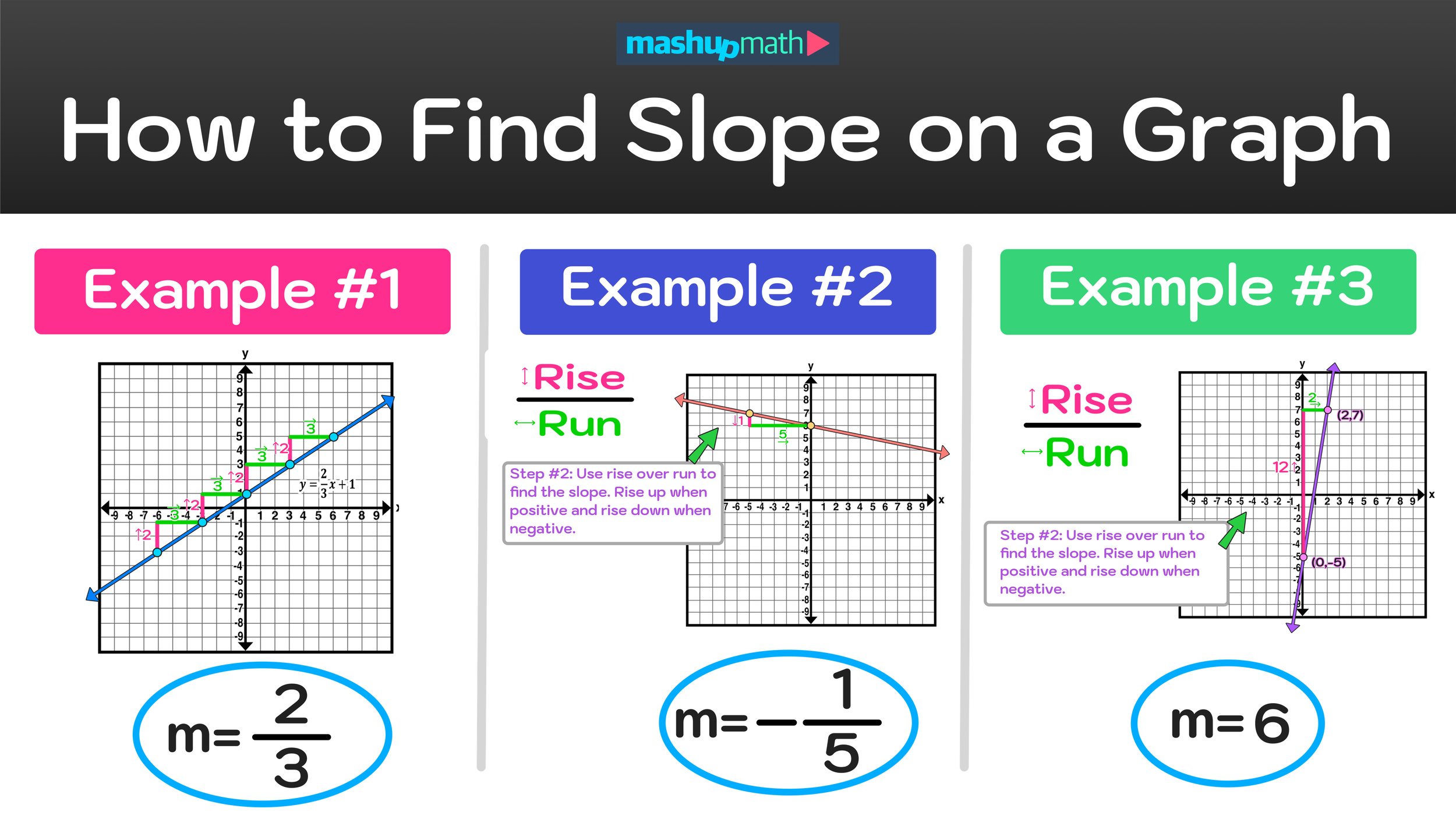
How to Find Slope on a Graph

Step-by-Step Guide: How to Find a Slope on a Graph by Following 3 Simple Steps

Step-by-Step Guide: How to find slope on a graph explained.

In algebra, you will often be working with linear functions of the form y=mx+b where m represents the slope and b represents the y-intercept.

When it comes to dealing with these types of linear functions on the coordinate plane, you can find figure out the slope of the line simply by analyzing its graph. This particular skill will be the focus of the free step-by-step guide, where we will learn how to find slope on a graph using a simple 3 step strategy.

This free guide on How to Find a Slope on a Graph will teach you everything you need to know about finding the slope of a line on a graph and this skill can be used to solve any problem that requires you to find the slope of a linear function graphed on the coordinate plane.

This guide will cover the following topics/sections:

• What is Slope? (Quick Review)

• How to Find Slope on a Graph Example #1

• How to Find Slope on a Graph Example #2

• How to Find Slope on a Graph Example #3

You can use the hyper-links above to jump to a particular section of this guide, or you can work through each section in order (this approach is highly recommended if you are learning this skill for the first time).

Are you ready to get started? Let’s begin with a quick review of slope.

Preview: In this guide, we will learn to use “rise over run” to find slope on a graph.

Quick Review—What is Slope?

Before we get into any examples of how to find a slope on a graph, it’s important that you understand the concept of slope and what it means.

Definition: The slope of a line refers to the direction and steepness of the line.

Slope is often expressed as a fraction where the numerator represents the vertical change (the change in y-position) and the denominator represents the horizontal change (the change in x-position). When a slope is a whole number, you can think of it as having a denominator of 1 (for example, a line with a slope of 4 actually has a slope of 4/1).

There are four types of slope:

• Positive Slope ↗️: Lines that increase from left to right have a positive slope.

• Negative Slope ↘️: Lines that decrease from left to right have a negative slope.

• Zero Slope ↔️: Horizontal lines have a slope of zero.

• Undefined Slope ↕️: Vertical lines have an undefined slope.

Since we will be dealing with finding slope on a graph in this guide, it is important that you are familiar with what these four kinds of slope look like. Before moving forward, take a close look Figure 01 below, which illustrates examples of these four kinds of slope.

Figure 01: There are four types of slope on a graph: positive, negative, zero, and undefined.

We often refer to slope in terms of “rise over run” where rise refers to the line’s vertical behavior and run refers to the line’s horizontal behavior.

In this guide, we will use “rise over run” to help us to find a slope on a graph.

So, how does “rise over run” work?

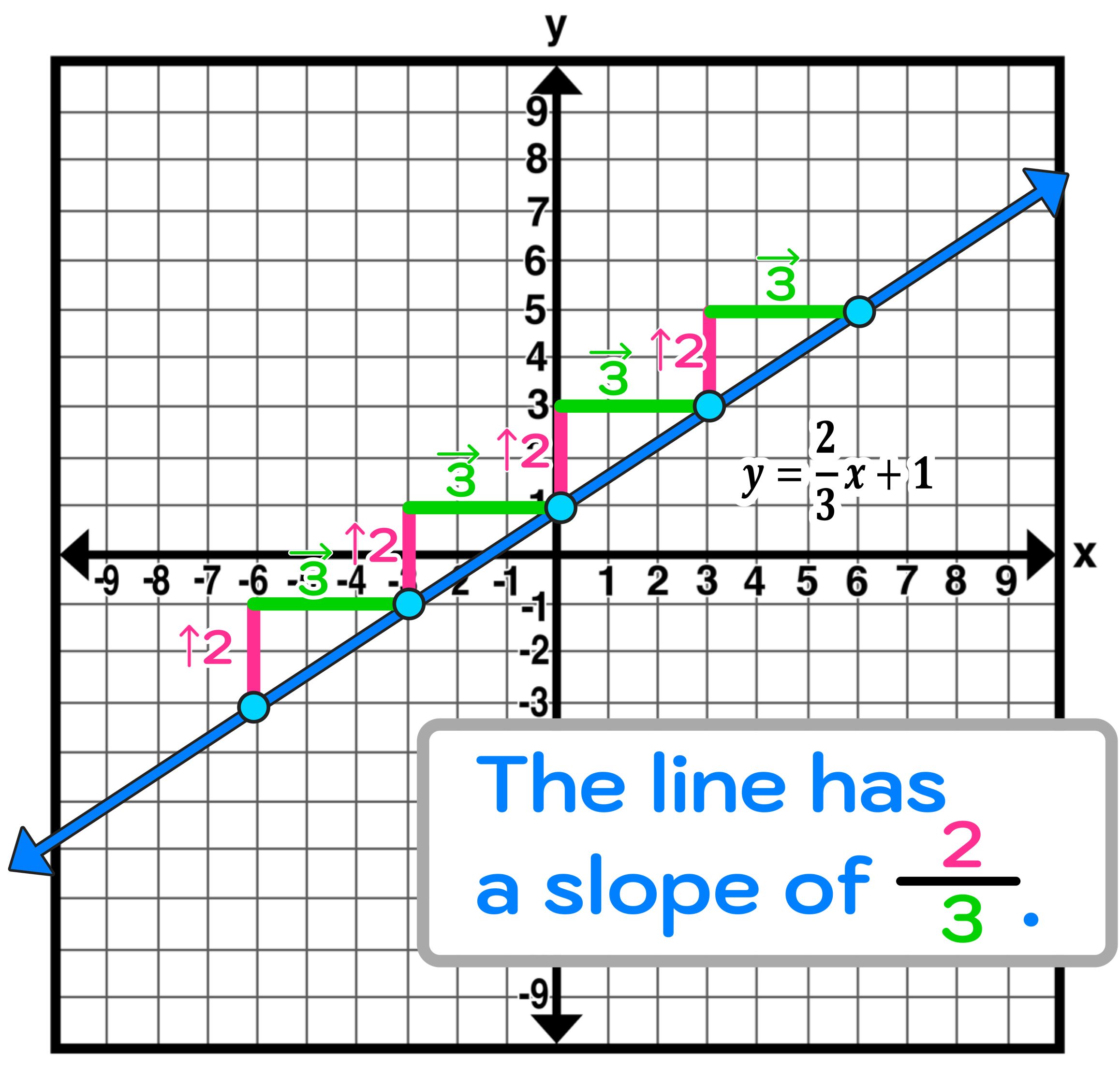
Let’s consider the graph in Figure 02 below.

Figure 02: How can we find the slope of the line y=2/3x+1 on the graph using rise over run?

First, we are given the graph of the line that represents the equation y=2/3x+1.

By looking at this graph, you can see that the line is increasing from left to right, so we know that the slope will be positive.

Also, notice that, in this case, we are given the equation of the line in y=mx+b form: y=2/3x+1, so we should already know that the slope will equal 2/3.

But, what if we just given the graph of the line without the equation? How then could we find the slope of the graph?

This is where rise over run comes into play. When you have a graph with at least two known points on the graph, you can use rise over run to “build a staircase” from one point to another to determine the slope of the line (i.e. find the fraction that represents the change in y-position over the change in x-position for the given line).

Figure 03 below illustrates how to use rise over run to build a staircase from point to point to find the slope of the line.

Figure 04: How to find slope of a line on a graph using rise over run.

Notice that our staircase consistently rises upwards two units and then runs 3 units to the right from point to point.

This tells us that the line has a slope of 2/3. And, since 2/3 can’t be simplified or reduced, we can conclude that the line on the graph has a slope of 2/3 (which is positive).

Note that not all slopes will be positive and it won’t always be the case that your resulting rise over run fraction can’t be simplified or reduced (we will see both occurrences in the examples ahead).

The key takeaways here are that:

• There are four types of slope: positive, negative, zero, and undefined

• Slope can be expressed as a fraction that represents “change in y” over “change in x”

• We can rise over run to find the slope of a graph as long as we know at least two points on the graph

Now, let’s go ahead and work through some examples of how to find a slope on a graph using an easy 3 step strategy that utilizes rise over run.

Figure 05: Understanding the difference between positive slopes and negative slopes in reference to rise over run.

---

How to Find Slope on a Graph

Example #1: Find the Slope of the Graph

For the first example and all of the examples that follow, we will use the following 3-step strategy for how to find a slope on a graph:

• Step #1: Select two coordinate points on the graph that have integer coordinates and plot them on the line clearly.

• Step #2: Using rise over run, build a step that connects the two points to find the change in y and the change in x (i.e. the slope of the line).

• Step #3: Express your answer as a fraction and simplify if possible.

Now, let’s go ahead and dive into this first practice problem where we are given a line and we are tasked with finding its slope.

Figure 06: Find the domain and range of the graph of y=x^2.

All that we are given is a line on the coordinate plane without any points or an equation. However, we can still determine the slope of the graph by applying our 3-steps as follows:

Step #1: Select two coordinate points on the graph that have integer coordinates and plot them on the line clearly.

To complete the first step, look for points where the graph intersects perfectly at a coordinate with integer coordinates (i.e. it crosses a point where four boxes meet). You can several options for this first example, but for this demonstration, we will choose the following points and plot them on the graph:

• (-5,7) and (0,6)

In Figure 07 below, you can see how we plotted these two points on the line to complete Step #1.

Figure 07: How to Find Slope on a Graph: The first step is to find and plot two points on the line with integer coordinates.

Step #2: Using rise over run, build a step that connects the two points to find the change in y and the change in x (i.e. the slope of the line).

Now we are ready to apply rise over run to find the slope. Starting with the leftmost point, we have to build a step that will connect the two points.

Notice that this line is decreasing from left to right, which means that the line has a negative slope.

Whenever we have a negative slope like the one in this example, we will have to “rise down” when performing rise over run (i.e. move downwards vertically instead of upwards).

The process for completing Step #2 is shown in Figure 08 below.

Figure 08: Since this line has a negative slope (it decreases from left to right), our rise action was in a downwards vertical direction).

Using rise over run, we can see that this negative slope rises downwards 1 unit and to the right 5 units, so we can conclude that the slope is -1/5.

Step #3: Express your answer as a fraction and simplify if possible.

We now have a fraction that represents the slope of this line: m = -1/5.

Since this slope was negative, it needs to include the negative sign. Now, the last step is to check if the fraction -1/5 can be simplified or reduced. Since it can not be, we can conclude that:

Final Answer: The line has a slope of -1/5.

If we were to use this result to “continue the staircase,” we will see that rising down 1 unit and running to the right 5 units from any point on the line will land you on another point on the line (as shown in Figure 09 below).

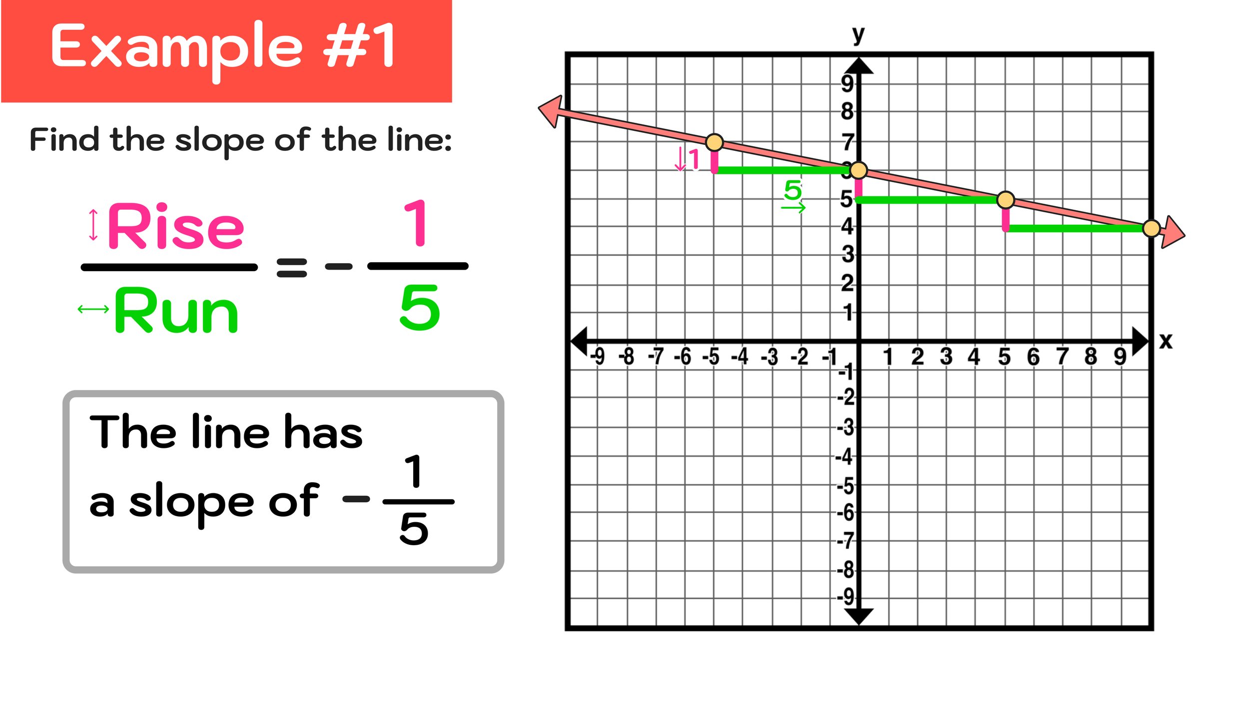
Figure 09: The line has a slope of -1/5.

You can use the 3-step strategy that we used for Example #1 to solve any problem where you have to find slope on a graph without a given equation. Let’s gain more experience with the 3-steps by working through another practice problem.

---

Example #2: Find the Slope of the Graph

For our next example, we have to find the slope of a graph of a pretty steep line. Notice that this line is increasing from left to right, so the slope will be positive.

Figure 10: How to Find the Slope of a Line on a Graph

Step #1: Select two coordinate points on the graph that have integer coordinates and plot them on the line clearly.

For the first step, let’s go ahead and find two points with integer coordinates that the line passes through. For this practice problem, we will choose the following points on the line:

• (0,-5) and (2,7)

Then go ahead and plot these points on the graph as shown in Figure 12 below:

Figure 12: To find the slope on a graph, start by plotting two points on the line that have integer coordinates.

Now that we have plotted our two points on the graph, we are ready for the next step.

Step #2: Using rise over run, build a step that connects the two points to find the change in y and the change in x (i.e. the slope of the line).

Next, we have to use rise over run and build a step that connects the two points so we can determine the slope.

Again, since this line is increasing from left to right, we know that the slope will be positive and that, unlike the last example where the slope was negative, we will have to “rise up” when performing rise over run.

Figure 13 below shows how we can use rise over run to get from (0,-5) to (2,7). You can see that the slope, in this case, is 12/2.

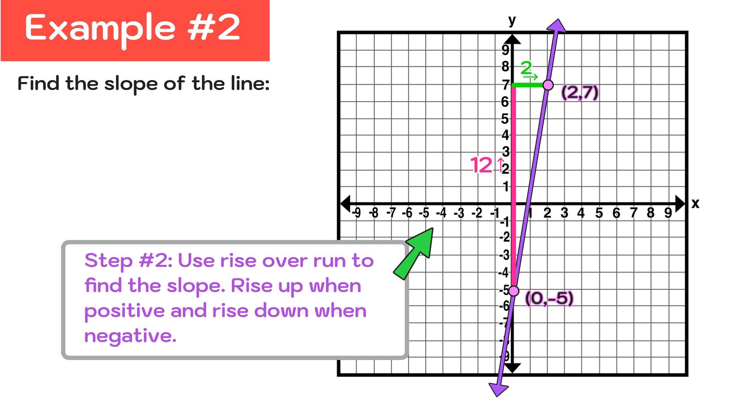
Figure 13: In this case, rise over run gives us a slope of 12/2, but can it be simplified?

After completing Step #2, we can see that the rise was 12 and the run was 2, so we conclude that our slope is: m = 12/2.

Is this our final answer? Let’s perform the third and final step to find out.

Step #3: Express your answer as a fraction and simplify if possible.

Although we have an answer in the form of a fraction, m=12/2, we should know that the fraction 12/2 can be simplified as 6/1 (or just 6).

To say that this line has a slope of 12/2 is not incorrect, but slopes of lines are typically expressed in reduced form.

If we apply our new slope of 6/1 to the point (0,-5) and build our staircase, we will see that the point (1,1) is also on the graph. And, if we continue from that point, we will end up at (2,7), which we know is also a point on the line.

The equivalent relationship between m=12/2 and m=6 is shown in Figure 14 below:

Figure 14: The slope 12/2 can be simplified as 6/1 or just 6.

Final Answer: The line has a slope of 6.

Are you starting to get the hang of it?

Let’s go ahead and take a look at another example.

---

Example #3: Find the Slope of the Graph

In this third example, let’s take a look at a horizontal line.

Figure 15: How to Find Slope on a Graph: Horizontal Lines

In our review of slope at the start of this guide, we shared that there are four kinds of slope: positive, negative, zero, and undefined.

In the case of horizontal lines, like the line shown on the graph in Figure 15 above, the slope will always be zero.

While we already know that the slope of this line is 0, let’s apply our 3-step method to see if this is actually true.

Step #1: Select two coordinate points on the graph that have integer coordinates and plot them on the line clearly.

You can pick any two points on the line. We will go with:

• (-4,6) and (5,6)

These points have been plotted on the graph in Figure 16 below:

Figure 16: How to find a slope on a graph: zero slope

Step #2: Using rise over run, build a step that connects the two points to find the change in y and the change in x (i.e. the slope of the line).

Notice that we can not rise or nor rise down since the slope of this line is neither negative nor positive.

Figure 17 below shows how we can use rise over run to get from (-4,6) to (5,6). Since the rise is 0 and the run is 6, we can say that the line has a slope of 0/6.

Figure 17: Horizontal lines have a slope of zero.

Step #3: Express your answer as a fraction and simplify if possible.

After completing Step #2, we know that the rise over run is 0/9, and we also know that 0 divided by 9 is just equal to 0 and we can conclude that:

Final Answer: The line has a slope of 0.

---

Conclusion: How to Find a Slope on a Graph

The slope of a line refers to the direction and steepness of that line and there are four types of slopes:

• Positive Slope ↗️

• Negative Slope ↘️

• Zero Slope ↔️

• Undefined Slope ↕️

You can find the slope on a graph of a line by using the rise over run approach and by following the following 3-step strategy:

• Step #1: Select two coordinate points on the graph that have integer coordinates and plot them on the line clearly.

• Step #2: Using rise over run, build a step that connects the two points to find the change in y and the change in x (i.e. the slope of the line).

• Step #3: Express your answer as a fraction and simplify if possible.

You can use these 3 steps to find the slope of any line on a graph, so make sure that you are comfortable using them before moving on. If you feel like you need more help, we recommend going back and working through the practice problems again!

Keep Learning:

How to Find Slope Using the Slope Formula

Your simple step-by-step guide to the formula for slope and how to use it to solve problems.

---

How to Find Scale Factor in 3 Easy Steps

How to Find Scale Factor in 3 Easy Steps

Step-by-Step Guide: How to Find the Scale Factor of a Dilation

Step-by-Step Guide: How to find scale factor of a dilation in 3 easy steps.

When learning about geometry transformations on the coordinate plane, dilations can be tricky since they are the only transformation that involves changing the shape of the original figure. In the case of dilating a figure, we use something called scale factor to determine whether to stretch a figure (make it larger) or shrink a figure (make it smaller) as well as by what factor.

This free step-by-step guide on How to Find Scale Factor in 3 Easy Steps will teach you how to determine the scale factor of a given dilation by looking at its graph and/or a given set of coordinate points.

This guide will cover the following topics:

• What is a Dilation?

• What is Scale Factor?

• How to Find Scale Factor Example #1

• How to Find Scale Factor Example #2

• How to Find Scale Factor Example #3

You can use the quick-links above to skip to any section of this guide. However, if are new to finding the scale factor a dilation, we recommend working through each section in order.

Now, let’s start off with a quick review of dilations and the definition of scale factor.

Figure 01: This guide will teach you how to find the scale factor of a dilation.

What is a Dilation?

Before we learn how to find the scale factor of a dilation, it’s important that we understand what a dilation is in the first place.

There are four types of transformations in geometry:

• Rotations: When you turn the object clockwise or counter-clockwise about a given point

• Reflections: When you create a mirror image of the original shape across a line of symmetry

• Translations: When you slide a figure from one location on the coordinate plan to another

• Dilations: When you stretch or shrink the image of a figure based on a given scale factor

This guide will focus on the fourth type of transformation—dilations.

Definition: Dilation

In math, a dilation refers to a transformation that results in a figure changing in size, but not shape. This means that the new figure will be made larger or smaller to the original figure, but it will remain proportional.

Figure 02: ▵A’B’C’ is formed after dilating ▵ABC by a scale factor greater than one.

Figure 02 above illustrates an example of a dilation where the image of ▵ABC is being stretched to form the new larger ▵A’B’C’.

Notice, however, that both triangles have the same shape and are proportional to each other. ▵A’B’C’ is just a scaled up version of ▵ABC.

What is Scale Factor?

Definition: Scale Factor

Every dilation is based on a scale factor, which we will denote using the letter k in this guide.

In math, a scale factor refers to the ratio between the side lengths and coordinate points of two similar figures. In the case of dilations, scale factor is used to describe by what factor the original image has been stretched (enlarged) or shrunk (reduced) in size.

When the scale factor, k, is greater than one, the result is an enlargement. When the scale factor, k, is less than one, the result is a reduction.

Figure 03 illustrates the relationship between an image and its scale factor in terms of the new image being larger or smaller.

Figure 03: When the scale factor is greater than one, the image will be stretched. When the scale factor is less than one, the image will be shrunk.

Note that the scale factor of a dilation must always be positive (i.e. the scale factor can never be zero or a negative number). Scale factors, however, can be equal to fractions (which we will see more of later on).

The key takeaway here is that the scale factor of a dilation is what tells you if an image is being made larger (stretched) or smaller (shrunk) and by what factor.

Now, let’s take a closer look at the dilation shown in Figure 01 above to see if we can figure out the scale factor in our first example below:

---

How to Find Scale Factor in 3 Easy Steps

Now that you are familiar with the key concepts and definitions associated with dilations and scale factor, you are ready to learn how to find the scale factor of a dilation using the following simple steps:

• Step 01: Determine the coordinates of a point on the original figure and the coordinates of the coordinates of the corresponding point on the new dilated figure.

• Step 02: Divide the x-value of the new figure coordinate by the x-value of the original figure coordinate to find the scale factor.

• Step 03: Repeat Step 02 using the y-values to confirm your answer.

Are you ready to try out our 3-step method for finding the scale factor of a dilation? Let’s go ahead and apply these steps to solving our first problem.

Example #1: How to Find the Scale Factor

For our first example, we have to find the scale factor that was used to dilated ▵ABC onto ▵A’B’C.

Figure 04: How to Find the Scale Factor of a Dilation.

For starters, we know than the original image is ▵ABC and the new image is ▵A’B’C’. Notice that the new image is larger than the original image, so we should expect our resulting scale factor to be greater than one.

Let’s go ahead and apply our three steps to see if this is the case:

Step 01: Determine the coordinates of a point on the original figure and the coordinates of the coordinates of the corresponding point on the new dilated figure.

For the first step, we can select any point on the original image, ▵ABC. In this case, let’s select point B with coordinates (2,3). The corresponding point on ▵A’B’C’ is point B’ with coordinates at (6,9).

• Original Image Point: B (2,3)

• Corresponding Point on New Image: B’ (6,9)

Note that you could have chosen points A and A’ or points C and C’. As long as you are consistent, you will be able to find the scale factor.

Step 02: Divide the x-value of the new figure coordinate by the x-value of the original figure coordinate to find the scale factor.

Next, we have to take the x-value of the point from the new figure (point B’) and divide it by the x-value of the corresponding point on the original figure (point B), as follows:

• The x-value of Point B’ at (6,9) is 6

• The x-value of Point B at (2,3) is 2

• 6 ➗ 2 = 3

Now we can conclude that our result is the value of our scale factor, so we can say that:

• The scale factor is 3.

Figure 05: The scale factor is 3, which means that ▵A’B’C’ is three times as large as ▵ABC.

When we concluded that the scale factor is 3, we are saying that ▵A’B’C’ is three times as large as ▵ABC.

This should make sense by looking at the graph and by remembering that we were expecting to have a scale factor greater than one in the first place. However, to ensure that we are correct, let’s go ahead and complete the third and final step.

Step 03: Repeat Step 02 using the y-values to confirm your answer.

Finally, we have to take the y-value of the point from the new figure (point B’) and divide it by the y-value of the corresponding point on the original figure (point B), as follows:

• The y-value of Point B’ at (6,9) is 9

• The y-value of Point B at (2,3) is 3

• 9 ➗ 3 = 3

We got the same answer! Now, we can conclude that:

Final Answer: The scale factor is 3.

It’s okay if you are still a little confused. Let’s go ahead and work through another example where we will find the scale factor of a dilation using our 3-steps.

---

Example #2: How to Find the Scale Factor

For this second example, we are again tasked with finding the scale factor of a dilation.

Figure 04: How to Find the Scale Factor of a dilation where the original image has been shrunk.

In this example, we can see that the new image of ▵S’U’V’ is the result of shrinking ▵SUV (since ▵S’U’V’ is smaller than ▵SUV). So, we know that our scale factor should be less than one.

We can now use of 3-steps to find the exact scale factor as follows:

Step 01: Determine the coordinates of a point on the original figure and the coordinates of the coordinates of the corresponding point on the new dilated figure.

Again, you can choose any point that you like as long as you are consistent. In this case, let’s choose point S on ▵SUV with coordinates at (-8,8). The corresponding point on ▵S’U’V’ is point S’ with coordinates at (-4,4).

• Original Image Point: S (-8,8)

• Corresponding Point on New Image: S’ (-4,4)

Step 02: Divide the x-value of the new figure coordinate by the x-value of the original figure coordinate to find the scale factor.

For the next step, let’s take the x-value of the point from the new figure (point S’) and divide it by the x-value of the corresponding point on the original figure (point S), as follows:

• The x-value of Point S’ at (-4,4) is -4

• The x-value of Point S at (-8,8) is -8

• -4 ➗ -8 = 1/2

Now we can conclude that our result is the value of our scale factor, so we can say that:

• The scale factor is 1/2.

Figure 05: How to find the scale factor that ▵SUV onto ▵S’U’V’.

A scale factor of 1/2 means that the original figure, ▵SUV, was shrunk down to half of its size to create the image of ▵S’U’V’.

Before we can confirm that our answer is correct, however, let’s complete the third and final step.

Step 03: Repeat Step 02 using the y-values to confirm your answer.

For step number three, we must take the y-value of the point from the new figure (point S’) and divide it by the y-value of the corresponding point on the original figure (point S), as follows:

• The y-value of Point S’ at (-4,4) is 4

• The y-value of Point S at (-8,8) is 8

• 4 ➗ 8 = 1/2

Notice that our result, again, is 1/2, so we can say that:

Final Answer: The scale factor is 1/2.

Are you starting to get the hang of it? Let’s go ahead to work through another example.

---

Example #3: How to Find the Scale Factor

Let’s go ahead and use our 3-step method to solve this final example.

Figure 06: How to Find the Scale Factor of a Dilation in 3 Easy Steps.

We can use the same 3-step method that we did on the previous two examples to solve this problem.

Notice that the new image of ▵Q’R’S’ is the result of shrinking the original image of ▵QRS, so our scale factor should be less than one.

Step 01: Determine the coordinates of a point on the original figure and the coordinates of the coordinates of the corresponding point on the new dilated figure.

Just like the last two examples, you can choose any point that you like as long as you are consistent. However, for this problem, we will intentionally avoid points Q and Q’ since they both have zero as coordinate points, which could cause problems since we can’t have zero in a denominator.

Instead, let’s choose point R on ▵QRS with coordinates at (9,3). The corresponding point on ▵Q’R’S’ is point R’ with coordinates at (3,1).

• Original Image Point: R (9,3)

• Corresponding Point on New Image: R’ (3,1)

Step 02: Divide the x-value of the new figure coordinate by the x-value of the original figure coordinate to find the scale factor.

Moving on, we have to take the x-value of the point from the new figure (point R’) and divide it by the x-value of the corresponding point on the original figure (point R), as follows:

• The x-value of Point R’ at (3,1) is 3

• The x-value of Point R at (9,3) is 9

• 9 ➗ 3 = 1/3

So, we have just figured out the ▵QRS was shrunk by a scaled factor of 1/3 to get the image of ▵Q’R’S’.

• The scale factor is 1/3.

In other words, ▵Q’R’S’ is one-third the size of ▵QRS.

Figure 07: How to Find Scale Factor: The scale factor is 1/3.

All that we have to do now is confirm that our answer is correcting by completing the third step.

Step 03: Repeat Step 02 using the y-values to confirm your answer.

To confirm that the scale factor was 1/3 is correct, we have to take the y-value of the point from the new figure (point R’) and divide it by the y-value of the corresponding point on the original figure (point R), as follows:

• The y-value of Point R’ at (3,1) is 1

• The y-value of Point R at (9,3) is 3

• 1 ➗ 3 = 1/3

Now that our answer has been confirmed, we can make the following conclusion:

Final Answer: The scale factor is 1/3.

---

Conclusion: How to Find Scale Factor

Understanding how to determine the scale factor of a dilation is an important geometry and algebra skill that every student must master when they are learning about transformations on the coordinate plane.

This step-by-step guide of finding scale factor reviewed the definition of a dilation on the coordinate plane and the meaning of scale factor in regards to dilations. When a scale factor, k, is greater than one, the resulting image is larger than the original image. And, when the scale factor, k, is less than one, the resulting images is smaller than the original image.

To solve problems where you are tasked with finding the scale factor of a dilation, we applied the following three step strategy:

• Step 01: Determine the coordinates of a point on the original figure and the coordinates of the coordinates of the corresponding point on the new dilated figure.

• Step 02: Divide the x-value of the new figure coordinate by the x-value of the original figure coordinate to find the scale factor.

• Step 03: Repeat Step 02 using the y-values to confirm your answer.

You can use these three steps to solve any problem where you are tasked with finding the scale factor of a dilation between two figures on the coordinate plane.

Keep Learning:

How to Perform Dilations on the Coordinate Plane

Learn how to perform dilations on the coordinate plane.

---

How to Find Domain and Range of a Graph—Step-by-Step

How to Find Domain and Range of a Graph Explained

Step-by-Step Guide: How to Find Domain and Range of a Graph Function, How to Find the Domain and Range of a Graph

Step-by-Step Guide: How to find domain and range of a graph explained.

In algebra, every function can be represented as a graph on the coordinate plane. The graph of a function provides a visually representation of how the function behaves and gives you important information—including its domain and range.

This free Step-by-Step Guide on How to Find Domain and Range of a Graph Function will teach you everything you need to know about finding the domain and range of function by looking at its graph and it includes the following sections:

• What is Interval Notation?

• What is the Domain and Range of a Function?

• How to Find Domain and Range of a Graph Example #1

• How to Find Domain and Range of a Graph Example #2

• How to Find Domain and Range of a Graph Example #3

• How to Find Domain and Range of a Graph Example #4

You can click on any of the quick links above to jump to a section, but we highly recommend that you work through each section in order to get the most out of this free guide.

Now, let’s do a quick review of some important vocabulary terms and concepts that you will need to be familiar with in order to learn how to find the domain and range of a graph.

Figure 01: Before you can learn how to find the domain and range of a graph, you have to be familiar with interval notation.

What is Interval Notation?

Before we review the meaning of domain and range and how to find domain and range of a graph, it is important that you are familiar with interval notation.

Interval Notation is used to describe a certain set of numbers using either parenthesis or square brackets.

• Square Brackets: When an endpoint is included in a given set of numbers, we use square brackets that look like [ or ].

• Parenthesis: When an endpoint is not included in a given set of numbers, we use parenthesis that look like ( or ).

In this section, we will use simple inequalities to teach you to understand interval notation. We will then extend this understanding to using interval notation when finding the domain and range of a graph.

Let’s consider the inequality x>4 as shown on the graph in Figure 02 below.

• Notice that all numbers greater than 4, but not including 4, are solutions to this inequality.

• Also notice that the arrow extends to the right forever towards infinity and that there an infinite number of values that would satisfy this inequality (i.e. there are an infinite amount of numbers that are greater than 4.

Figure 02: The inequality x>4 (x is greater than 4) on the number line.

We could express the solution to the inequality x>4 verbally as:

• x is greater than 4 (i.e. x can be any number greater than 4, but not including 4)

And we could express the solution to the inequality x>4 using interval notation as:

• (4,∞)

Notice that, since 4 was not included in the solution set, we used parenthesis instead of square brackets.

Now let’s consider the inequality x≥4 as shown on the graph in Figure 03 below.

Figure 03: The inequality x≥4 (x is greater than or equal to 4) on the number line.

Notice that all numbers greater than 4, and including 4, are solutions to this inequality.

We could express the solution to the inequality x≥4 verbally as:

• x is greater than or equal to 4 (i.e. x can be 4 or any number greater than 4)

And we could express the solution to the inequality x>4 using interval notation as:

• [4,∞)

Notice that, since 4 was included in the solution set, we used square brackets instead of parenthesis.

The difference between the solutions to x>4 and x≥4 in interval notation are summarized in Figure 04 below. The key takeaway here is that you use parentheses when the endpoint is a number and is not included in the solution set and square brackets when the endpoint is a number and is included in the solution set.

Figure 04: Use parentheses when the endpoint is a number and is not included in the solution set and square brackets when the endpoint is a number and is included in the solution set.

Did you notice that you only have to differentiate between parentheses and brackets when the endpoint is a number?

In the case of infinity, you will always use parentheses since ∞ is not a definitive value or a true endpoint.

Next, let’s take a look at one more inequality: x ≤ 0 as shown on the graph in Figure 05 below:

Figure 05: The inequality x≤0 (x is less than or equal to 0) on the number line.

Notice that all numbers less than 0, and including 0, are solutions to this inequality.

We could express the solution to the inequality x≤0 verbally as:

• x is less than or equal to 0 (i.e. x can be 0 or any number less than 0)

And we could express the solution to the inequality x≤0 using interval notation as:

• (-∞,0]

When using interval notation, we have to identify the smallest value(s) on the left side and the largest on the right side. So, in this case of x≤0, we have to state on the left side that the smallest values are approaching negative ∞ and, on the right, the largest possible value is 0 (and, since 0 is included the solution set, we have to use a square bracket).

Figure 06 below illustrates a few more examples of the solutions of inequalities expressed in interval notation. Make sure that you are comfortable with interval notation before moving forward, as it is key to learning how to find domain and range of a graph function.

Figure 06: How to find domain and range of a graph starts with understanding interval notation.

---

What is Domain and Range?

Domain

In algebra, the domain of a function refers to the set of all possible x-values for that function.

For example, the function y=x² has a domain of (-∞,∞). This means that the domain includes all real numbers since any number can be squared (positive, negative, or zero) without any limitations.

Range

In algebra, the range of a function refers to the set of all possible y-values for that function.

For example, the function y=x² has a range of [0,∞) because any number squared, whether positive or negative, will always be greater than or equal to zero (the result can never be negative).

Figure 07: The domain of a function refers to the set of all possible x-values and the range refers to all possible y-values.

Now that you are familiar with interval notation and the meaning of domain and range, let’s go ahead and look at our first example.

For example #1, we will look at the graph of the function y=x². As previously stated, we already know the domain and range of y=x² are:

• The domain of y=x² is (-∞,∞)

• The range of y=x² is [0,∞)

Let’s see how we can verify that we are correct simply by looking at the graph of y=x².

---

How to Find Domain and Range of a Graph

Example #1: Find the Domain and Range of a Graph

For our first example, we are given the graph of the function f(x)=x^2 and we are tasked with finding the domain and the range (note that our answers must be in interval notation).

Figure 08: Find the domain and range of the graph of y=x^2.

Remember that the domain refers to all of the possible x-values, and the range refers to all of the possible y-values.

Let’s start with finding the domain of this graph. Notice that the graph is a parabola that extends forever on both the left and right-side of zero. This means that, as far as the x-axis is concerned, that the graph will extend forever to the left towards negative infinity and towards the right forever towards positive infinity.

What does mean? The graph will eventually cross through every possible value of x without any exceptions or limitations.

So, we can conclude that the domain of this function is (-∞,∞), as shown in Figure 09 below:

Figure 09: The domain of the graph is (-∞,∞), meaning that the graph will pass through every possible x-value.

Next, let’s find the range. Remember that the range refers to all of the possible y-values that the graph passes through.

Unlike the domain, the graph clearly will not pass through every possible y-value. The lowest y-value of this particular graph is the vertex, or turning point, of the parabola, which is at the origin.

So, the smallest possible y-value for this graph is 0 and the largest is infinity since it continues forever and ever in an upwards direction.

So, we can conclude that the range of this function is [0,∞), as shown in Figure 10 below:

Figure 10: The range of the graph is [0,∞), meaning that the graph will pass through every possible y-value that is greater than or equal to 0.

Now, we have confirmed that the function y=x^2 has a domain and range of:

• Domain: (-∞,∞)

• Range: [0,∞)

Now let’s move onto another example where we gain more experience with how to find domain and range of a graph.

---

Example #2: Find the Domain and Range of a Graph

For our next example, we have to find the domain and range of the graph of the function f(x)=-|x|.

Figure 11: How to Find the Domain and Range of a Graph Example #2

The domain of the graph refers to all of the possible x-values.

Just like the previous example, the graph will pass cross through every possible x-value without any exceptions or limitations, so we can conclude that:

• Domain: (-∞,∞)

The range of the graph refers to all of the possible y-values.

Notice that this graph is similar to the graph in Example #1, except it is upside down. As far as the range is concerned, this graph has an upper limit at 0 and a lower limit at negative infinity since it extends forever and ever in a downward direction, so we can conclude that:

• Range: (-∞,0]

Figure 12: The graph has a domain of (-∞,∞) and a range of (-∞,0].

In conclusion, the graph y=-|x| has the following domain and range:

• Domain: (-∞,∞)

• Range: [0,∞)

Are you starting to get the hang of it? Let’s continue onto the next example.

---

Example #3: Find the Domain and Range of a Graph

For our third example, let’s find the domain and range of the graph of f(x)=(1/4)x^3

Figure 13: How to Find Domain and Range of a Graph

Since this graph extends forever and ever in both directions left and right, we know that the domain of the graph will be all real numbers and we can conclude that:

• Domain: (-∞,∞)

Similarly, the graph also extends forever and ever in both directions up and down, so we know that the range of the graph will also be all real numbers and we can conclude that:

• Range: (-∞,∞)

Figure 14: Both the domain and range of the graph are (-∞,∞).

Final Answer: The domain and range of a graph with equation f(x)=(1/4)x^3 is:

• Domain: (-∞,∞)

• Range: [0,∞)

---

Example #4: Find the Domain and Range of a Graph

Moving on, we have to find the domain and range of the graph of f(x)=√(x+6)

Figure 15: How to find the domain range of a graph of f(x)=√(x+6)

The graph in our fourth example involves a function with a square root. Notice that, unlike the first three examples, the domain has some limitations.

Namely, the domain starts at -6 and extends forever to the right. So, in this case, the domain is not all real numbers. Rather, the domain is:

• Domain: [-6,∞)

And, the range also has limitations and is not all real numbers. Notice that the y-values start at zero and extend forever in an upward direction, so we can conclude that the range is:

• Range: [0,∞)

Figure 16: How to find the domain and range of a function graph explained.

Final Answer: The graph of the function f(x)=√(x+6) has a domain and range of:

• Domain: [-6,∞)

• Range: [0,∞)

---

Conclusion: How to Find Domain and Range of a Graph

Being able to identify the domain and range of a graph function and expressing the domain and range using interval notation are important and useful algebra skills.

In this free guide, we learned the definitions of the domain and range of a function, how to describe the domain and range of a function using interval notation, and how to find the domain and range of a graph of a function.

Key takeaways:

• Domain and range are expressed using interval notation. When an endpoint is included in, we use square brackets and, when it is not, we use parentheses. Whenever -∞ or ∞ is an endpoint, we use parentheses.

• Domain and range, when expressed using interval notation, always puts the smallest value/endpoint on the left and the largest value/endpoint on the right.

• The domain of a function refers to the set of all possible x-values for that function and the range of a function refers to all of the possible y-values for that function.

• When determining the domain of a function by looking at its graph, you need to look at its horizontal behavior (how it travels across the x-axis in both positive and negative directions).

• When determining the range of a function by looking at its graph, you need to look at its vertical behavior (how it travels across the y-axis in both positive and negative directions).

That’s all there is to it! If you still confused about how to find the domain and range of a graph, we highly recommend going back and working through the practice problems again.

Keep Learning:

How to Find the Vertex of a Parabola in 3 Easy Steps

Learn how to find the coordinates of the vertex point of any parabola with this free step-by-step guide.

---

How to Factor Quadratic Equations—Step-by-Step Examples and Tutorial

How to Factor Quadratic Equations Explained

Step-by-Step Guide: How to Factor a Quadratic Equation, How to Solve Quadratic Equations by Factoring

Step-by-Step Guide: How to factor a quadratic equation explained.

In algebra, a quadratic equation is an equation of the form ax² + bx + c = 0 where a can not equal zero.

The word quad is Latin for four or fourth, which is why a quadratic equation has four terms (ax², bx, c, and 0). Being able to solve quadratic equations by factoring is an incredibly important algebra skill that every student will need to learn in order to be successful in Algebra I, Algebra II, and beyond. Learning how to factor a quadratic equation comes down to being able to recognize a quadratic equation, being able to factor it, and then finally being able to solve for x and check your answer for mistakes.

This free Step-by-Step Guide on How to Factor Quadratic Equations will cover the following topics:

• What is a Quadratic Equation?

• What are the Solutions of a Quadratic Equation?

• How to Factor Quadratic Equations when a=1

• How to Factor Quadratic Equations when a≠1?

Note that this guide is a follow-up to our free step-by-step guide How to How to Factor Polynomials, which reviews how to factor polynomials with 2 terms, 3 terms, and 4 terms. While we will review general factoring in this guide, we will be more focused on how to factor a quadratic equation.

However, before we learn how to factor quadratic equations and how to solve quadratic equations by factoring, let’s quickly review some important vocabulary terms related to quadratics and quadratic equations.

Figure 01: What is the difference between a trinomial expression and a quadratic equation.

What is a Trinomial Expression?

While the focus of this guide is on teaching you how to factor quadratic equations and how to solve quadratic equations by factoring, it is important that you first understand how the difference between a trinomial expression and a quadratic equation.

In algebra, a trinomial expression is a polynomial with 3 terms of the form ax² + bx + c. Note that, since it is an expression, a trinomial does not include an equal sign.

• ax² + bx + c

What is a Quadratic Equation?

In algebra, a quadratic equation is a trinomial of the form ax² + bx + c that is equal to zero. So, we can say that a quadratic equation is of the form:

• ax² + bx + c = 0

Figure 01 above illustrates this key difference between trinomial expressions and quadratic equations, which is namely that a quadratic equation is an equation and includes a fourth term (=0).

Why are we concerned with quadratic equations being equal to zero? You may already know that, when graphed, quadratic equations can be represented on the coordinate plane as a parabola (a U-shaped curved). When we solve quadratic equations by factoring, we are actually figuring out where the parabola crosses zero on the x-axis, as shown in Figure 02 below.

Figure 02: By setting a quadratic equation equal to zero, we are able to determine where the parabola crosses the x-axis. These x-values will be the solution(s) to a quadratic equation. This guide will teach you how to solve quadratic equations by factoring (not graphing).

Consider the example quadratic in Figure 02 above:

• x² +6x + 8 = 0

Notice that, for this quadratic equation, a=1, b=6, and c=8. When it comes time to learn how to factor a quadratic equation later on, it will be important that you are able to identify the values of a, b, and c for any given quadratic equation.

Now, here are two key pieces of information about the solutions to quadratic equations:

• The solution(s) to any quadratic equation are the points where the graph of the quadratic crosses the x-axis on a graph.

• Quadratic equations typically have two solutions, but they can also have one solution or zero solutions.

• You do not have to graph quadratic functions to solve them. You can solve quadratic equations by factoring.

Now that you understand what the solutions of a quadratic represent graphically, you are ready to learn how to factor equations and solve them algebraically.

Are you ready to get started?

---

How to Factor Quadratic Equations: Intro

Let’s start by factoring the example quadratic equation from Figure 02 above: x² +6x + 8 = 0

Example #1: Factor and Solve x² +6x + 8 = 0

From our graph, we already know that this quadratic equation will have two solutions: x=-4 and x=-2 (note that this can also be written as x={-4,-2}). So, let’s use factoring to find these answers algebraically.

To factor a quadratic equation, we can split it up into two parts:

• The left side of the equal sign

• The right side of the equal sign

On the left side of the equal sign, we must have a trinomial of the form ax² + bx + c to deal with and, on the right side, we must have a zero. If the quadratic equation in question is not in this form, we will have to use algebra to rearrange it. However, this first example is good to go so we don’t have to move any of the terms around. This first step is shown in Figure 03 below:

Figure 03: How to factor a quadratic equation.

From here, the next step is to factor the trinomial on the left side of the equal sign:

• x² +6x + 8

Note that, for this introductory example, the value of a (the leading coefficient) is 1. When this is the case, you can factor the trinomial on the left-side of the equation as follows:

Figure 04: How to solve quadratic equations by factoring.

Step One: Identify the values of b and c.

In this example, the values of b and c are: b=6 & c=8

Step Two: Find two numbers that both ADD to b and MULTIPLY to c.

Once you have identified the values of b and c (6 and 8 respectively in this example), you can use trial-and-error to find two numbers that both add to the b term (6) and multiply to the c term (8). Another way to say this is: find two numbers with a sum of 6 and a product of 8.

For example, let’s say that you chose the numbers 5 and 1. In this case, 5+1=6, but 5x1≠ 8, so these two numbers would not work.

• 5 + 1 =6 (the value of b) ✓

• 5 x 1 ≠ 8 (the value of c) ✘

However, if you chose the numbers 2 and 4:

• 2 + 4 =6 (the value of b) ✓

• 2 x 4 = 8 (the value of c) ✓

Since the sum of 2 and 4 is 6 and the product of 2 and 4 is 8, you can found out that the factors of the trinomial x² + 6x + 8 are (x+2) and (x+4)

Step Three: Use your numbers from step two to write out the factors

In this case, you can conclude that the factors of x² + 6x + 8 are (x+2) and (x+4).

Figure 05: x² + 6x + 8 = (x+2)(x+4).

How do you know if you result is correct? You can check your answer by performing double distribution as follows:

• (x+2)(x+4) = x² + 2x + 4x + 8 = x² + 6x + 8

If the result is the same trinomial that you started with, then you know that your factors are correct.

Figure 06: How to Solve a Quadratic Equation by Factoring

Now we have a new equation:

• (x+4)(x+2)=0

This is not our final answer. To solve this quadratic by factoring, we have to take each factor, set it equal to zero, and solve to find our solutions as follows:

• x+4 = 0 → x = -4

• x+2 = 0 → x = -2

Figure 07: The final step is to set each factor equal to zero and solve.

Final Answer: The quadratic equation x² + 6x + 8=0 has a solution of x={-4,-2}.

This solution should make sense since we already knew from the graphing the parabola that this particular quadratic would equal zero at x=-4 and x=-2.

Now that Example #1 is complete, you know exactly how to factor quadratic equations and how to solve quadratic equations by factoring. However, the way that you factor will vary by problem as not all trinomials are factored the same way.

Below, you will find examples for how to solve a quadratic equation by factoring for three different occasions:

• when the leading coefficient a=1 (this applies to Example #1)

• when the leading coefficient a≠1

For a more in-depth review of factoring trinomials, we highly recommend visiting our popular Step-by-Step Guide to Factoring Polynomials. Otherwise, let’s continue on to learning how to factor quadratic equations when a=1.

---

How to Factor Quadratic Equations When a=1

For this first section, we will focus on how to factor a quadratic equation with a leading coefficient of 1 (as opposed to any other number). Figure 08 highlights the difference between a quadratic equation where a=1 and a quadratic equation where a≠1.

Figure 08: Make sure that you can recognize when a quadratic has a leading coefficient of one or not.

Example #2: Factor and Solve x² -2x -15 = 0

First, note that this quadratic equation is in the form ax² + bx + c = 0 since the equation could be rewritten as:

• x² + (-2x) + (-15) =0

However, for the sake of simplicity, we will keep it as:

• x² -2x -15 =0

Since a=1 in this example, we can solve this quadratic equation the same way we solved Example #1.

First, we can split the quadratic into two parts: the left-side of the equal sign and the right-side of the equal sign. Then we can attempt to factor the trinomial x² -2x -15 on the left-side.

Figure 09: How to Factor Quadratic Equations: Start by isolating the trinomial on the left-side of the equal sign.

Now, we can find the factors of x² -2x -15 as follows:

Step One: Identify the values of b and c.

In this example, the values of b and c are: b=-2 & c=-15

Step Two: Find two numbers that both ADD to b and MULTIPLY to c.

Once you have identified the values of b and c (-2 and -15 respectively in this example), you can use trial-and-error to find two numbers that both add to the b term (-2) and multiply to the c term (-15). Another way to say this is: find two numbers with a sum of -2 and a product of -15.

In cases like this example, you need two number that will multiply to a -15. Since the product of two negatives is always positive and the product of two positives is also always positive, your factors will include one positive number and one negative number.

After some trial-and-error, you will find that 3 and -5 work because:

• 3 + -5 = -2 (the value of b) ✓

• 3 x -5 = -15 (the value of c) ✓

Since the sum of 3 and -5 is -2 and the product of 3 and -5 is -15, you have found out that the factors of the trinomial x² -2x -15 are (x+3) and (x-5)

Step Three: Use your numbers from step two to write out the factors

In this case, you can conclude that the factors of x² -2x -15 are (x+3) and (x-5).

Figure 10: Factor the trinomial on the left-side of the equal sign.

From here, we have a new equation to deal with:

• (x+3)(x-5)=0

To find the solution(s) to the original quadratic equation, we have to take each factor, set it equal to zero, and solve for x as follows:

• x+3 = 0 → x = -3

• x-5 = 0 → x = 5

Figure 11: How to Solve a Quadratic Equation by Factoring

Final Answer: The quadratic equation x² - 2x - 15 =0 has a solution of x={-3,5}.

Now, let’s look at one more example of how to factor quadratic equations when the leading coefficient is 1.

---

Example #3: Factor and Solve x² + 4x = 12

Do you notice anything different about this next example?

The equation is not a quadratic (i.e. it is not in ax² +bx + c = 0 form). To get this equation into ax² +bx + c = 0, we will have to rearrange it, namely by subtracting 12 from both sides so that there is a zero on the right side of the equals sign as follows:

• x² + 4x = 12

• x² + 4x -12 = 12 -12

• x² + 4x -12 = 0

By rearranging the terms in this way, our new equation is a quadratic that is now in ax² +bx + c = 0 form, meaning that we can solve it by factoring.

Figure 12: How to Factor a Quadratic Equation

Now, we can find the factors of x² +4x -12 as follows:

Step One: Identify the values of b and c.

In this example, the values of b and c are: b=4 & c=-12

Step Two: Find two numbers that both ADD to b and MULTIPLY to c.

Once you have identified the values of b and c (4 and -12 respectively in this example), you can use trial-and-error to find two numbers that both add to the b term (4) and multiply to the c term (-12). Another way to say this is: find two numbers with a sum of 4 and a product of -12.

After some trial-and-error, you will find that 6 and -2 work because:

• 6 + —2 = 4 (the value of b) ✓

• 6 x —2 = -12 (the value of c) ✓

Step Three: Use your numbers from step two to write out the factors

In this case, you can conclude that the factors of x² + 4x -12 are (x+6) and (x-2).

Finally, we can find our solutions by solving

• (x+6)(x-2)=0

To find the solution(s) to the original quadratic equation, we have to take each factor, set it equal to zero, and solve for x as follows:

• x+6 = 0 → x = -6

• x-2 = 0 → x = 2

Final Answer: The quadratic equation x² + 4x - 12 = 0 has a solution of x={-6,2}.

The entire step-by-step process for solving this example is illustrated in Figure 12 above. Now let’s move onto learning bow to factor a quadratic equation when the leading coefficient is not equal to one.

---

How to Factor Quadratic Equations When a≠1

Example #4: Factor and Solve 2x² - x - 6 = 0

For the first example, we have to find the solutions to the quadratic equation: 2x² - x - 6 = 0.

Notice that, in this case, the leading coefficient a≠1 (in this example a=2).

We can still solve this quadratic equation by separating the left and right-side of the equal sign where the trinomial is on the left side and the zero is on the right side as shown in Figure 13 below.

Figure 13: How to Factor a Quadratic Equation when a≠1

Now, we have to find the factors of the trinomial 2x² - x - 6 on the left-side of the equal sign as follows:

Figure 14: How to factor a trinomial a≠1

Factoring these types of trinomials is a bit more involved.

First, notice that you can not pull out a greatest common factor (GCF). When this is the case, you can use the AC method for factoring trinomials of the form ax² + bx + c when a≠1 as follows:

Step One: Identify the values of a and c and multiply them together

For this example, a=2 and c=-6…

• a x c = 2 x -6 = -12

Step Two: Factor and replace the middle term

Next, you have to take the resulting product from Step One (-12) and use it as a replacement for the middle term.

This means that you are replacing the middle term, -1x, with -12x, which we then have to factor as follows:

• -12 = -4 x 3; and

• -4 + 3 = -1

We chose -4 and 3 as factors because the sum of -4 and 3 equals negative 1, so we can rewrite the original trinomial as 2x² - 4x +3x - 6, as shown in Figure 15 below.

Figure 15: How to use the AC method to factor

Step Three: Split the new polynomial down the middle and take the GCF of each side

Our new polynomial is equivalent to the one that we started with, but now it has four terms: 2x² - 4x + 3x - 6

Now, you must split the polynomial down the middle to essentially create two separate binomials that you can simplify by dividing GCF’s out of as follows:

• First Binomial: 2x² - 4x = 2x(x-2)

• Second Binomial: 3x - 6 = 3(x-2)

This process of splitting the polynomial down the middle is illustrated in Figure 16 below.

Figure 16: Split the new polynomial down the middle and take the GCF of each side

Step Four: Identify the Factors

Lastly, you can now determine the factors.

The result from the previous step was 2x(x - 2) + 3(x -2). Within this expression you will find your two factors, (2x+3) and (x-2), as shown in Figure 17 below.

Figure 17: How to Factor Quadratic Equations

And now, you can conclude that the factors of 2x² - x - 6 are (2x+3) and (x-2).

Unfortunately, you still have to set these factors equal to zero and solve for x to find the solution to the original quadratic equation as follows:

• 2x + 3 = 0 → 2x = -3 → x = -3/2

• x-2 = 0 → x = 2

Final Answer: The quadratic equation 2x² - x - 6 = 0 has a solution of x={ -3/2 , 2 }.

The complete step-by-step process for solving this final example is illustrated in Figure 18 below.

Figure 18: How to Factorize Quadratic Equations

---

Conclusion: How to Solve Quadratic Equations by Factoring

Learning how to factor quadratic equations is a key algebra skill that can be learned with practice.

While many students will initially learn how to solve quadratic equations by graphing, the next step will be to learn how to solve quadratic equations by factoring, which means that you will have to know how to factor quadratic of the form ax² + bx + c = 0 when a=1 and when a≠1.

In this step-by-step guide to factoring quadratic equations, we covered both cases as we worked through several examples of factoring quadratics of the form ax² + bx + c = 0. Remember that not all questions will be directly in this form, but they can often be rearranged (i.e. they can be rewritten as an equivalent equation that is in the form ax² + bx + c = 0).

If you are still confused about how to factor quadratic equations, we highly recommend that you go back and work through all of the example problems above, carefully following each step. The more experience that you have working on these types of problems, the easier they will become.

Keep Learning:

How to Factor Polynomials (Free Step-by-Step Guide)

Learn how to factor binomials, trinomials, and cubic expressions.

---

How to Divide Decimals Explained—Step-by-Step Examples and Tutorial

How to Divide Decimals Explained in 3 Easy Steps

Step-by-Step Guide: How to Divide Decimals by Whole Numbers and How to Solve Decimal Divided by Decimal Problems

Free Step-by-Step Guide: Dividing Decimals Explained in 3 Easy Steps

In math, it is important to be able to work with and perform operations on decimals, which are numbers in the base-10 system that include a point that separates the whole number(s) from the attached fractional parts. For example, the number 2.5 is a decimal number that represents two and a half.

One of the more challenging operations to perform with decimals is division. However, if you know how to divide whole numbers, then you can easily learn how to divide decimals using just a few simple steps. Note that there are two different cases when it comes to dividing decimals: a decimal divided by a whole number and a decimal divided by another decimal. We will cover both cases in this guide.

Below are quick links to each section of this free Step-by-Step Guide on How to Divide Decimals:

• Quick Review: What is a Dividend? What is a Divisor?

• Quick Review: Long Division

• How to: Divide Decimals by Whole Numbers

• How to: Dividing Decimals by Decimals

• Extra Practice: Free Dividing Decimals Worksheet

While learning how to divide with decimals can be intimidating at first, it is a math skill that you can easily learn with practice following a simple 3-step process. This free dividing with decimals tutorial will teach you everything you need to know about how to divide with decimals, including several step-by-step practice problems for both dividing decimals by whole numbers and dividing decimals by decimals.

But, before we dive into our practice problems, let’s do a quick recap of some important vocabulary terms related to division as well as a quick review of how to perform long division. If you are already comfortable with the review information, you can use the quick links above to skip ahead to the section that best meets your needs.

Figure 01: How to Divide Decimals: Key Vocabulary

What is a dividend? What is a divisor?

In this guide on dividing decimals, we will be using the terms dividend and divisor often, so make sure that you are familiar with what they mean:

• When dividing two numbers, the dividend is the number that is being divided.

• When dividing two numbers, the divisor is the number of parts the dividend is being divided into.

For example, consider the division problem: 248 ÷ 8

• 248 is the dividend because it is the number being divided

• 8 is the divisor because 248 is being divided into 8 parts.

This example is illustrated in Figure 01 above.

Because this guide will be teaching you how to divide decimals without using a calculator, we will be using long division to solve problems. Therefore, it is important that you are familiar with the divisor/dividend notation shown in Figure 01 above, where: 248 ÷ 8 → 8 | 248

Now that you know how to identify a dividend and a divisor and the divisor/dividend notation, lets do a quick review of how to perform long division using the same example of 248 ÷ 8.

Figure 02: Dividing Decimals Explained: Long Division Review

Figure 02 above shows a step-by-step review of how to use long division to determine that 248 ÷ 8 = 31.

If you are not comfortable with performing long division, then we recommend that you pause now and do a deeper review before moving forward with this tutorial on how to divide decimals.

---

How to Divide Decimals by Whole Numbers

The first set of examples in this dividing decimals tutorial will focus on how to divide decimals by whole numbers and will include examples for when the dividend is the whole number and when the divisor is the whole number as well.

How to Divide Decimals by Whole Numbers

Example #1: 1.5 ÷ 2

Let’s start off with a simple example that you could probably solve without the use of long division (although we will solve it using long division anyway so that you can start to become more familiar with our 3-step process for dividing decimals).

For this example, and all of the examples that follow, you will be using the following three step method for dividing decimals:

• Step One: Identify the dividend and the divisor and determine whether or not the divisor is a whole number (if it is, move onto Step Three).

• Step Two: If the divisor is not a whole number, multiply it by a multiple of 10 to make it a whole number (multiply tenths by 10, hundredths by 100, thousandths by 1,000, etc.). Whatever multiple of 10 that you multiplied the divisor by, you must also multiply the dividend by.

• Step Three: Use long division to solve.

We will be applying this 3-step process of all of the dividing decimals practice problems in this guide, so don’t get intimidated if you are a little confused right now. The process will make more sense and be easier to apply after we work through a few examples.

Figure 03: How to Divide Decimals: First, identify whether or not the divisor is a whole number.

Lets start with the first step:

Step One: Identify the dividend and the divisor and determine whether or not the divisor is a whole number (if it is, move onto Step Three).

In the case of 1.5 ÷ 2

• 2 is the divisor

• 1.5 is the dividend

As shown in Figure 03 above, it is clear that the divisor is 2, which is indeed a whole number, so, for this example, we can skip the second step and move right onto Step Three.

Also notice that in Figure 03 above, we rewrote 1.5 as 1.50 (they both mean the same thing). Adding extra zeros after the last digit of a decimal does not change the number and often helps you to perform long division, as you will see in the next step.

Step Three: Use long division to solve.

All that you have to do now is use long division to solve the problem. You can click play on the video below to see an animated step-by-step breakdown of how to perform the long division for this problem.

Based on the video and the illustrated summary shown in Figure 04 below, you can see that:

Solution: 1.50 ÷ 2 = 0.75

This solution should make sense because dividing 1.50 in half will result in 0.75. Before moving onto another similar example of a decimal divided by a whole number, we encourage you to review the above review as we will not include videos for every example.

Figure 04: How to Divide Decimals by Whole Numbers: Example #1 Solved

---

Dividing Decimals by Whole Numbers

Example #2: 24.36 ÷ 3

For this next example, we will be using the exact same three-step approach as Example #1.

Step One: Identify the dividend and the divisor and determine whether or not the divisor is a whole number (if it is, move onto Step Three).

For this example:

• 3 is the divisor

• 24.36 is the dividend

Since the divisor in this example is a whole number (3), we can skip the second step just like we did in the previous example and move onto the third and final step.

Step Three: Use long division to solve.

To solve the second example, perform long division just as you did to solve Example #1. Remember to follow your steps carefully and to line up your decimal points.

The entire process of using long division to solve 24.36 ÷ 3 is illustrated in Figure 05 below.

Figure 05: Dividing decimals by whole numbers explained.

After completing Step Three, we can conclude that:

Solution: 24.36 ÷ 3 = 8.12

Now, lets look at a few examples of a decimal divided by a whole number where the divisor is not a whole number.

---

How to Divide Decimals by Whole Numbers

Example #3: 92 ÷ 2.3

For this third example of dividing decimals by whole numbers, we will again be using the same three-step method as the previous two examples (as well as all on the examples that will follow this one), except that this time we will not be able to skip the second step.

Step One: Identify the dividend and the divisor and determine whether or not the divisor is a whole number (if it is, move onto Step Three).

In this case:

• 2.3 is the divisor

• 92 is the dividend

Since the divisor in this example is 2.3, which is not a whole number, we will have to move onto the second step (which we were able to skip in the previous two examples).

Step Two: If the divisor is not a whole number, multiply it by a multiple of 10 to make it a whole number (multiply tenths by 10, hundredths by 100, thousandths by 1,000, etc.). Whatever multiple of 10 that you multiplied the divisor by, you must also multiply the dividend by.

When it comes to dividing decimals, we cannot have a decimal as a divisor. However, we can multiply both the divisor and the dividend by the same multiple of ten to transform the divisor into a whole number and still have a proportional relationship.

Since the final digit of 2.3 is in the tenths place value slot, we will multiply both the divisor (2.3) and the dividend (92) by 10 as shown below and in Figure 06:

• 2.3 x 10 = 23

• 92 x 10 = 920

*Remember that what you do to one number, you must do to the other number. If you forget to multiply both the dividend and the divisor by 10, you will get the wrong answer.

Figure 06: How to Divide Decimals by Whole Numbers: The divisor has to be a whole number.

Step Three: Use long division to solve.

After completing Step Two, all we have to do is use long division to solve 920 ÷ 23.

The step-by-step process for using long division to divide 920 by 23 is shown in Figure 07 below.

Figure 07: Decimal divided by a whole number

Finally, we can say that:

Solution: 92 ÷ 2.3 = 40

Next, lets look at one final example of how to divide decimals by whole numbers before we move onto learn all about dividing decimals by decimals.

How to Divide Decimals by Whole Numbers

Example #4: 16 ÷ 6.25

Step One: Identify the dividend and the divisor and determine whether or not the divisor is a whole number (if it is, move onto Step Three).

For the fourth example, the divisor is a decimal and the dividend is a whole number.

• 6.25 is the divisor

• 16 is the dividend

Step Two: If the divisor is not a whole number, multiply it by a multiple of 10 to make it a whole number (multiply tenths by 10, hundredths by 100, thousandths by 1,000, etc.). Whatever multiple of 10 that you multiplied the divisor by, you must also multiply the dividend by.

Since the divisor is a decimal (6.25), we will have to multiply both the divisor and the dividend by the same multiple of ten.

And since, in this example, the final digit of the divisor, 6.25, is in the hundredths place value slot, we will multiply both the divisor and the dividend by 100 as shown below and in Figure 08.

• 6.25 x 100 = 625

• 16 x 100 = 1,600

Figure 08: How do you divide decimals by whole numbers?

After completing long division, we can conclude that:

Solution: 16 ÷ 6.25 = 2.56

Now we will move on from dividing decimals by whole numbers to learning how to divide decimals by decimals.

---

Dividing Decimals by Decimals

This section of our guide focused on dividing decimals by decimals. If you used the quick links at the top of the page to skip to this section, we recommend working through the examples in the dividing decimals by whole numbers section above, because it will help you to better understand how to use the following three-step method for dividing decimals by decimals:

• Step One: Identify the dividend and the divisor and determine whether or not the divisor is a whole number (if it is, move onto Step Three).

• Step Two: If the divisor is not a whole number, multiply it by a multiple of 10 to make it a whole number (multiply tenths by 10, hundredths by 100, thousandths by 1,000, etc.). Whatever multiple of 10 that you multiplied the divisor by, you must also multiply the dividend by.

• Step Three: Use long division to solve.

Just as the previous section on dividing decimals by whole numbers, we will be following the same steps for dividing decimals by decimals.

Lets go ahead and dive into the first example.

---

How to Divide with Decimals

Example #1: 7.68 ÷ 0.4

Step One: Identify the dividend and the divisor and determine whether or not the divisor is a whole number (if it is, move onto Step Three).

For this first example:

• 0.4 is the divisor

• 7.68 is the dividend

For all of the examples in this section, we will be dividing decimals by decimals, so it will always be the case that the divisor is not a whole number. Therefore, you will always have to move onto Step Two, where you will use multiplication to transform the divisor into a whole number.

Step Two: If the divisor is not a whole number, multiply it by a multiple of 10 to make it a whole number (multiply tenths by 10, hundredths by 100, thousandths by 1,000, etc.). Whatever multiple of 10 that you multiplied the divisor by, you must also multiply the dividend by.

Again, a decimal divided by a decimal can not be solve using long division when the divisor is not a whole number. Luckily, you can easily transform the divisor into a whole number by multiplying both the divisor and the dividend by a multiple of ten and still have a proportional relationship where you can use long division to solve the problem.

Since the final digit of 0.4 is in the tenths place value slot, you can multiply both the divisor (0.4) and the dividend (7.68) by 10 as shown below and as illustrated in Figure 09.

• 0.4 x 10 = 4

• 7.68 x 10 = 76.8

*Always remember that whenever you multiply the divisor by a multiple of 10, you also have to multiply the dividend by that same multiple of 10. If you forget to multiply both by the same multiple of 10, you will not be able to correctly solve the problem.

Figure 09: How to Divide with Decimals: Use multiples of 10 to transform the divisor into a whole number.

Step Three: Use long division to solve.

Now that you have transformed the divisor into a whole number, you can use long division to solve the problem. You can click play on the video below to see an animated step-by-step breakdown of how to perform the long division for this problem.

Based on the video and the illustrated summary shown in Figure 10 below, we can conclude that:

Solution: 7.68 ÷ 0.4 = 19.2

Before you continue onto the next example of how to divide decimals by decimals, we highly recommend that you review the step-by-step long division tutorial above as we will not include video tutorials for every problem.

Figure 10: How to divide decimals by decimals.

---

How to Divide Decimals by Decimals

Example #2: 38.4 ÷ 0.24

Just like the previous example, we will use our three step method to solve a decimal divided by a decimal problem.

Step One: Identify the dividend and the divisor and determine whether or not the divisor is a whole number (if it is, move onto Step Three).

For this first example:

• 0.24 is the divisor

• 38.4 is the dividend

Step Two: If the divisor is not a whole number, multiply it by a multiple of 10 to make it a whole number (multiply tenths by 10, hundredths by 100, thousandths by 1,000, etc.). Whatever multiple of 10 that you multiplied the divisor by, you must also multiply the dividend by.

Since the divisor, 0.24, is a decimal, you will have to multiply it (and the dividend) by a power of ten to make it a whole number. Since the last digit of 0.24 is in the hundredths place value slot, we will multiply both the divisor and the dividend by 100 as shown below and in Figure 11.

• 0.24 x 100 = 24

• 38.4 x 100 = 3,840

Figure 11: Solving a decimal divided by a decimal problems.

Step Three: Use long division to solve.

Finally, you now have a divisor that is a whole number, so you can simply use long division to solve 3,840 ÷ 24 to find the solution to this problem, as illustrated in Figure 12 below.

Figure 12: How to Divide Decimals Step-by-Step

Solution: 38.4 ÷ 0.24 = 160

Now, lets work through one final example.

---

How to Divide Decimals by Decimals

Example #3: 4.76 ÷ 1.36

Step One: Identify the dividend and the divisor and determine whether or not the divisor is a whole number (if it is, move onto Step Three).

For this first example:

• 1.36 is the divisor

• 4.76 is the dividend

Step Two: If the divisor is not a whole number, multiply it by a multiple of 10 to make it a whole number (multiply tenths by 10, hundredths by 100, thousandths by 1,000, etc.). Whatever multiple of 10 that you multiplied the divisor by, you must also multiply the dividend by.

Since the divisor, 1.36, is a decimal, you will have to multiply it (and the dividend) by 100 to transform it into a whole number (we chose to multiply the dividend and the divisor by 100 because the last digit of 1.36 is in the hundredths decimal slot).

• 1.36 x 100 = 136

• 4.76 x 100 = 476

Step Three: Use long division to solve.

Now you can find the solution by using long division to solve 476 ÷ 136 as shown in Figure 13 below.

Figure 13: Dividing decimals example #3 solution.

Solution: 4.76 ÷ 1.36 = 3.5

---

Dividing Decimals Worksheet

Are you looking for some extra practice with solving problems involving dividing decimals?

You can click the link below to download your free Dividing Decimals Worksheet, which includes a complete answer key so you can check your work. Be sure to apply the three-step process shared in this guide (and also featured on the worksheet) when solving the problems.

▶ Download Your Free Dividing Decimals Worksheet (w/ Answer Key)

▶ Access More Free Topic-Specific Math Worksheets

View fullsize

Dividing Decimals Worksheet Preview

Conclusion: How to Divide Decimals

Learning how to divide decimals by whole numbers or other decimals is an important math skill that every student will eventually have to learn how to do.

While dividing decimals can seem challenging, as long as you know how to perform long division, you can easily solve dividing decimals problems by using the following 3-step approach:

• Step One: Identify the dividend and the divisor and determine whether or not the divisor is a whole number (if it is, move onto Step Three).

• Step Two: If the divisor is not a whole number, multiply it by a multiple of 10 to make it a whole number (multiply tenths by 10, hundredths by 100, thousandths by 1,000, etc.). Whatever multiple of 10 that you multiplied the divisor by, you must also multiply the dividend by.

• Step Three: Use long division to solve.

By working through the examples in this guide as well as the practice problems on the free dividing decimals worksheet, you will gain invaluable practice and experience with dividing decimals, which will make solving problems where you have to divide decimals a simple and easy task.

---

Keep Learning:

How to Convert a Decimal to a Fraction in 3 Easy Steps (Free Step-by-Step Guide for Students)